Level-set method

The figure on the right illustrates several ideas about LSM. In the upper left corner is a bounded region with a well-behaved boundary. Below it, the red surface is the graph of a level set function determining this shape, and the flat blue region represents the X-Y plane. The boundary of the shape is then the zero-level set of , while the shape itself is the set of points in the plane for which is positive (interior of the shape) or zero (at the boundary).

In the top row, the shape's topology changes as it is split in two. It is challenging to describe this transformation numerically by parameterizing the boundary of the shape and following its evolution. An algorithm can be used to detect the moment the shape splits in two and then construct parameterizations for the two newly obtained curves. On the bottom row, however, the plane at which the level set function is sampled is translated upwards, on which the shape's change in topology is described. It is less challenging to work with a shape through its level-set function rather than with itself directly, in which a method would need to consider all the possible deformations the shape might undergo.

Thus, in two dimensions, the level-set method amounts to representing a closed curve (such as the shape boundary in our example) using an auxiliary function , called the level-set function. The curve is represented as the zero-level set of by

and the level-set method manipulates implicitly through the function . This function is assumed to take positive values inside the region delimited by the curve and negative values outside.

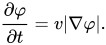
If the curve moves in the normal direction with a speed , then by chain rule and implicit differentiation, it can be determined that the level-set function satisfies the level-set equation

Here, is the Euclidean norm (denoted customarily by single bars in partial differential equations), and is time. This is a partial differential equation, in particular a Hamilton-Jacobi equation, and can be solved numerically, for example, by using finite differences on a Cartesian grid.

However, the numerical solution of the level set equation may require advanced techniques. Simple finite difference methods fail quickly. Upwinding methods such as the Godunov method are considered better; however, the level set method does not guarantee preservation of the volume and shape of the set level in an advection field that maintains shape and size, for example, a uniform or rotational velocity field. Instead, the shape of the level set may become distorted, and the level set may disappear over a few time steps. Therefore, high-order finite difference schemes, such as high-order essentially non-oscillatory (ENO) schemes, are often required, and even then, the feasibility of long-term simulations is questionable. More advanced methods have been developed to overcome this; for example, combinations of the leveling method with tracking marker particles suggested by the velocity field.

Consider a unit circle in , shrinking in on itself at a constant rate, i.e. each point on the boundary of the circle moves along its inwards pointing normally at some fixed speed. The circle will shrink and eventually collapse down to a point. If an initial distance field is constructed (i.e. a function whose value is the signed Euclidean distance to the boundary, positive interior, negative exterior) on the initial circle, the normalized gradient of this field will be the circle normal.

If the field has a constant value subtracted from it in time, the zero level (which was the initial boundary) of the new fields will also be circular and will similarly collapse to a point. This is due to this being effectively the temporal integration of the Eikonal equation with a fixed front velocity.

• In mathematical modeling of combustion, LSM is used to describe the instantaneous flame surface, known as the G equation.
• Level-set data structures have been developed to facilitate the use of the level-set method in computer applications.
• Computational fluid dynamics
• Trajectory planning
• Optimization
• Image processing
• Computational biophysics
• Discrete complex dynamics (visualization of the parameter plane and the dynamic plane)

The level-set method was developed in 1979 by Alain Dervieux, and subsequently popularized by Stanley Osher and James Sethian. It has since become popular in many disciplines, such as image processing, computer graphics, computational geometry, optimization, computational fluid dynamics, and computational biology.