Encyclopedia

Lenia

Continuous generalization of cellular automata

Wikipedia contributorsAdapted for Fathomly · View authors

4 min read
Source updated August 19, 2026

Image credit is listed at the end of this article.

Lenia is a family of cellular automata created by Bert Wang-Chak Chan. It is intended to be a continuous generalization of Conway's Game of Life, with continuous states, space and time. As a consequence of its continuous, high-resolution domain, the complex autonomous patterns ("lifeforms" or "spaceships") generated in Lenia are described as differing from those appearing in other cellular automata, being "geometric, metameric, fuzzy, resilient, adaptive, and rule-generic".

Lenia won the 2018 Virtual Creatures Contest at the Genetic and Evolutionary Computation Conference in Kyoto, an honorable mention for the ALIFE Art Award at ALIFE 2018 in Tokyo, and Outstanding Publication of 2019 by the International Society for Artificial Life (ISAL).

01Rules

Iterative updates

Let ${\mathcal {L}}$ be the lattice or grid containing a set of states $S^{\mathcal {L}}$ . Like many cellular automata, Lenia is updated iteratively; each output state is a pure function of the previous state, such that

$\Phi (A^{0})=A^{\Delta t},\Phi (A^{\Delta t})=A^{2\Delta t},\ldots ,\Phi (A^{t})=A^{t+\Delta t},\ldots$

where $A^{0}$ is the initial state and $\Phi :S^{\mathcal {L}}\rightarrow S^{\mathcal {L}}$ is the global rule, representing the application of the local rule over every site $\mathbf {x} \in {\cal {L}}$ . Thus $\Phi ^{N}(A^{t})=A^{t+N\Delta t}$ .

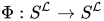
If the simulation is advanced by $\Delta t$ at each timestep, then the time resolution $T={\frac {1}{\Delta t}}$ .

State sets

Let $S=\{0,1,\ldots ,P-1,P\}$ with maximum $P\in \mathbb {Z}$ . This is the state set of the automaton and characterizes the possible states that may be found at each site. Larger $P$ correspond to higher state resolutions in the simulation. Many cellular automata use the lowest possible state resolution, i.e. $P=1$ . Lenia allows for much higher resolutions. Note that the actual value at each site is not in $[0,P]$ but rather an integer multiple of $\Delta p={\frac {1}{P}}$ ; therefore we have $A^{t}(\mathbf {x} )\in [0,1]$ for all $\mathbf {x} \in {\mathcal {L}}$ . For example, given $P=4$ , $\mathbf {A} ^{t}(\mathbf {x} )\in \{0,0.25,0.5,0.75,1\}$ .

Neighborhoods

Mathematically, neighborhoods like those in Game of Life may be represented using a set of position vectors in $\mathbb {R} ^{2}$ . For the classic Moore neighborhood used by Game of Life, for instance, ${\mathcal {N}}=\{-1,0,1\}^{2}$ ; i.e. a square of size 3 centered on every site.

In Lenia's case, the neighborhood is instead a ball of radius $R$ centered on a site, ${\mathcal {N}}=\{\mathbf {x} \in {\mathcal {L}}:\lVert \mathbf {x} \rVert _{2}\leq R\}$ , which may include the original site itself.

Note that the neighborhood vectors are not the absolute position of the elements, but rather a set of relative positions (deltas) with respect to any given site.

Local rule

There are discrete and continuous variants of Lenia. Let $\mathbf {x}$ be a vector in $\mathbb {R} ^{2}$ within ${\mathcal {L}}$ representing the position of a given site, and ${\mathcal {N}}$ be the set of sites neighboring $\mathbf {x}$ . Both variations comprise two stages:

Using a convolution kernel $\mathbf {K} :{\mathcal {N}}\rightarrow S$ to compute the potential distribution $\mathbf {U} ^{t}(\mathbf {x} )=\mathbf {K} *\mathbf {A} ^{t}(\mathbf {x} )$ .
Using a growth mapping $G:[0,1]\rightarrow [-1,1]$ to compute the final growth distribution $\mathbf {G} ^{t}(\mathbf {x} )=G(\mathbf {U} ^{t}(\mathbf {x} ))$ .

Once $\mathbf {G} ^{t}$ is computed, it is scaled by the chosen time resolution $\Delta t$ and added to the original state value: $\mathbf {A} ^{t+\Delta t}(\mathbf {x} )={\text{clip}}(\mathbf {A} ^{t}+\Delta t\;\mathbf {G} ^{t}(\mathbf {x} ),\;0,\;1)$ Here, the clip function is defined by $\operatorname {clip} (u,a,b):=\min(\max(u,a),b)$ .

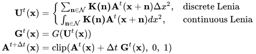
The local rules are defined as follows for discrete and continuous Lenia:

${\begin{aligned}\mathbf {U} ^{t}(\mathbf {x} )&={\begin{cases}\sum _{\mathbf {n} \in {\mathcal {N}}}\mathbf {K(n)} \mathbf {A} ^{t}(\mathbf {x} +\mathbf {n} )\Delta x^{2},&{\text{discrete Lenia}}\\\int _{\mathbf {n} \in {\mathcal {N}}}\mathbf {K(n)} \mathbf {A} ^{t}(\mathbf {x} +\mathbf {n} )dx^{2},&{\text{continuous Lenia}}\end{cases}}\\\mathbf {G} ^{t}(\mathbf {x} )&=G(\mathbf {U} ^{t}(\mathbf {x} ))\\\mathbf {A} ^{t+\Delta t}(\mathbf {x} )&={\text{clip}}(\mathbf {A} ^{t}(\mathbf {x} )+\Delta t\;\mathbf {G} ^{t}(\mathbf {x} ),\;0,\;1)\end{aligned}}$

Kernel generation

There are many ways to generate the convolution kernel $\mathbf {K}$ . The final kernel is the composition of a kernel shell $K_{C}$ and a kernel skeleton $K_{S}$ .

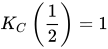
For the kernel shell $K_{C}$ , Chan gives several functions that are defined radially. Kernel shell functions are unimodal and subject to the constraint $K_{C}(0)=K_{C}(1)=0$ (and typically $K_{C}\left({\frac {1}{2}}\right)=1$ as well). Example kernel functions include:

$K_{C}(r)={\begin{cases}\exp \left(\alpha -{\frac {\alpha }{4r(1-r)}}\right),&{\text{exponential}},\alpha =4\\(4r(1-r))^{\alpha },&{\text{polynomial}},\alpha =4\\\mathbf {1} _{\left[{\frac {1}{4}},{\frac {3}{4}}\right]}(r),&{\text{rectangular}}\\\ldots ,&{\text{etc.}}\end{cases}}$

Here, $\mathbf {1} _{A}(r)$ is the indicator function.

Once the kernel shell has been defined, the kernel skeleton $K_{S}$ is used to expand it and compute the actual values of the kernel by transforming the shell into a series of concentric rings. The height of each ring is controlled by a kernel peak vector $\beta =(\beta _{1},\beta _{2},\ldots ,\beta _{B})\in [0,1]^{B}$ , where $B$ is the rank of the parameter vector. Then the kernel skeleton $K_{S}$ is defined as

$K_{S}(r;\beta )=\beta _{\lfloor Br\rfloor }K_{C}(Br{\text{ mod }}1)$

The final kernel $\mathbf {K} (\mathbf {n} )$ is therefore

$\mathbf {K} (\mathbf {n} )={\frac {K_{S}(\lVert \mathbf {n} \rVert _{2})}{|K_{S}|}}$

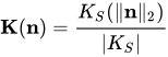
such that $\mathbf {K}$ is normalized to have an element sum of $1$ and $\mathbf {K} *\mathbf {A} \in [0,1]$ (for conservation of mass). $|K_{S}|=\textstyle \sum _{\mathcal {N}}\displaystyle K_{S}\,\Delta x^{2}$ in the discrete case, and $\int _{N}K_{S}\,dx^{2}$ in the continuous case.

Growth mappings

The growth mapping $G:[0,1]\rightarrow [-1,1]$ , which is analogous to an activation function, may be any function that is unimodal, nonmonotonic, and accepts parameters $\mu ,\sigma \in \mathbb {R}$ . Examples include

$G(u;\mu ,\sigma )={\begin{cases}2\exp \left(-{\frac {(u-\mu )^{2}}{2\sigma ^{2}}}\right)-1,&{\text{exponential}}\\2\cdot \mathbf {1} _{[\mu \pm 3\sigma ]}(u)\left(1-{\frac {(u-\mu )^{2}}{9\sigma ^{2}}}\right)^{\alpha }-1,&{\text{polynomial}},\alpha =4\\2\cdot \mathbf {1} _{[\mu \pm \sigma ]}(u)-1,&{\text{rectangular}}\\\ldots ,&{\text{etc.}}\end{cases}}$

where $u$ is a potential value drawn from $\mathbf {U} ^{t}$ .

Game of Life

The Game of Life may be regarded as a special case of discrete Lenia with $R=T=P=1$ . In this case, the kernel would be rectangular, with the function $K_{C}(r)=\mathbf {1} _{\left[{\frac {1}{4}},{\frac {3}{4}}\right]}(r)+{\frac {1}{2}}\mathbf {1} _{\left[0,{\frac {1}{4}}\right)}(r)$ and the growth rule also rectangular, with $\mu =0.35,\sigma =0.07$ .

02Patterns

By varying the convolutional kernel, the growth mapping and the initial condition, over 400 "species" of "life" have been discovered in Lenia, displaying "self-organization, self-repair, bilateral and radial symmetries, locomotive dynamics, and sometimes chaotic nature". Chan has created a taxonomy for these patterns.

Watch videos about LeniaExplainers and documentaries on YouTube (opens in a new tab)

Sources and credits

This article is adapted from the Wikipedia article “Lenia”, written by its contributors and licensed under CC BY-SA 4.0. Fathomly has changed the layout, removed citation markers, navigation and maintenance notices, and adjusted punctuation. This adapted version is shared under the same license. For references, see the original article.

Images, from Wikimedia Commons:

Lenia icon4.png by Bert Wang-Chak Chan, CC BY 4.0
Moore neighborhood.svg by MorningLemon, CC BY-SA 4.0
Lenia neighborhood.png by Bert Chan, CC BY-SA 4.0
Screenshot from 2021-10-12 18-26-15.png by Bert Chan, CC BY-SA 4.0
Lenia species.png by Bert Chan, CC BY-SA 4.0
Cellular automata and convnets.png by William Gilpin, CC BY-SA 4.0

Fathomly is not affiliated with or endorsed by the Wikimedia Foundation. Spotted a problem? Tell us.

Lenia

01Rules

Iterative updates

State sets

Neighborhoods

Local rule

Kernel generation

Growth mappings

Game of Life

02Patterns

Sources and credits

Related topics

Conway's Game of Life

Cellular automaton

Self-replication

Lenia

01Rules

Iterative updates

State sets

Neighborhoods

Local rule

Kernel generation

Growth mappings

Game of Life

02Patterns

03Related work

Sources and credits

Related topics

Conway's Game of Life

Cellular automaton

Self-replication