Encyclopedia

Brillouin and Langevin functions

Mathematical function, used to describe magnetization

Wikipedia contributorsAdapted for Fathomly · View authors

7 min read
Source updated September 6, 2026

The Brillouin and Langevin functions are a pair of special functions that appear when studying an idealized paramagnetic material in statistical mechanics. These functions are named after French physicists Paul Langevin and Léon Brillouin, who contributed to the microscopic understanding of magnetic properties of matter.

The Langevin function is derived using statistical mechanics and describes how magnetic dipoles are aligned by an applied field. The Brillouin function was developed later to give an explanation that considers quantum physics. The Langevin function could then be seen as a special case of the more general Brillouin function if the quantum number $J$ was infinite ( $J\to \infty$ ).

01Brillouin function for paramagnetism

The Brillouin function arises when studying magnetization of an ideal paramagnet. In particular, it describes the dependency of the magnetization $M$ on the applied magnetic field $B$ , defined by the following equation:

$B_{J}(x)={\frac {2J+1}{2J}}\coth \left({\frac {2J+1}{2J}}x\right)-{\frac {1}{2J}}\coth \left({\frac {1}{2J}}x\right)$

The function $B_{J}$ is usually applied in the context where $x$ is a real variable and a function of the applied field $B$ . In this case, the function varies from -1 to 1, approaching +1 as $x\to +\infty$ and -1 as $x\to -\infty$ .

The total angular momentum quantum number $J$ is a positive integer or half-integer. Considering the microscopic magnetic moments of the material. The magnetization is given by: $M=Ng\mu _{\text{B}}JB_{J}(x)$

where

$N$ is the number of atoms per unit volume,
$g$ the g-factor,
$\mu _{\text{B}}$ the Bohr magneton,
$x$ is the ratio of the Zeeman energy of the magnetic moment in the external field to the thermal energy $k_{\text{B}}T$ : $x=J{\frac {g\mu _{\text{B}}B}{k_{\text{B}}T}}$
$k_{\text{B}}$ is the Boltzmann constant and $T$ the temperature.

Note that in the SI system of units $B$ given in tesla stands for the magnetic field, $B=\mu _{0}H$ , where $H$ is the auxiliary magnetic field given in A/m and $\mu _{0}$ is the permeability of vacuum.

Click "show" to see a derivation of this law:
A derivation of this law describing the magnetization of an ideal paramagnet is as follows. Let z be the direction of the magnetic field. The z-component of the angular momentum of each magnetic moment (a.k.a. the azimuthal quantum number) can take on one of the 2J+1 possible values -J,-J+1,...,+J. Each of these has a different energy, due to the external field B: The energy associated with quantum number m is $E_{m}=-mg\mu _{\text{B}}B=-k_{\text{B}}Txm/J$ (where g is the g-factor, μ_B is the Bohr magneton, and x is as defined in the text above). The relative probability of each of these is given by the Boltzmann factor: $P(m)={\frac {1}{Z}}e^{-E_{m}/(k_{\text{B}}T)}={\frac {1}{Z}}e^{xm/J}$ where Z (the partition function) is a normalization constant such that the probabilities sum to unity. Calculating Z, the result is: $P(m)={\frac {e^{xm/J}}{\sum \limits _{m'=-J}^{J}e^{xm'/J}}}.$ All told, the expectation value of the azimuthal quantum number m is ${\begin{aligned}\langle m\rangle &=(-J)\times P(-J)+\cdots +J\times P(J)\\[1ex]&={\frac {\displaystyle \sum _{m=-J}^{J}me^{xm/J}}{\displaystyle \sum _{m=-J}^{J}e^{xm/J}}}.\end{aligned}}$ The denominator is a geometric series and the numerator is a type of arithmetico-geometric series, so the series can be explicitly summed. After some algebra, the result turns out to be $\langle m\rangle =JB_{J}(x)$ With N magnetic moments per unit volume, the magnetization density is $M=Ng\mu _{\text{B}}\langle m\rangle =NgJ\mu _{\text{B}}B_{J}(x).$

Click "show" to see a derivation of this law:

A derivation of this law describing the magnetization of an ideal paramagnet is as follows. Let z be the direction of the magnetic field. The z-component of the angular momentum of each magnetic moment (a.k.a. the azimuthal quantum number) can take on one of the 2J+1 possible values -J,-J+1,...,+J. Each of these has a different energy, due to the external field B: The energy associated with quantum number m is

$E_{m}=-mg\mu _{\text{B}}B=-k_{\text{B}}Txm/J$ (where g is the g-factor, μ_B is the Bohr magneton, and x is as defined in the text above). The relative probability of each of these is given by the Boltzmann factor: $P(m)={\frac {1}{Z}}e^{-E_{m}/(k_{\text{B}}T)}={\frac {1}{Z}}e^{xm/J}$ where Z (the partition function) is a normalization constant such that the probabilities sum to unity. Calculating Z, the result is: $P(m)={\frac {e^{xm/J}}{\sum \limits _{m'=-J}^{J}e^{xm'/J}}}.$ All told, the expectation value of the azimuthal quantum number m is ${\begin{aligned}\langle m\rangle &=(-J)\times P(-J)+\cdots +J\times P(J)\\[1ex]&={\frac {\displaystyle \sum _{m=-J}^{J}me^{xm/J}}{\displaystyle \sum _{m=-J}^{J}e^{xm/J}}}.\end{aligned}}$ The denominator is a geometric series and the numerator is a type of arithmetico-geometric series, so the series can be explicitly summed. After some algebra, the result turns out to be $\langle m\rangle =JB_{J}(x)$ With N magnetic moments per unit volume, the magnetization density is $M=Ng\mu _{\text{B}}\langle m\rangle =NgJ\mu _{\text{B}}B_{J}(x).$

High-field saturation limit

When $x\to \infty$ , the Brillouin function goes to 1. The magnetization saturates with the magnetic moments completely aligned with the applied field:

$M=Ng\mu _{\text{B}}J$

Low field/high-temperature limit

For low fields the curve appears almost linear, and could be replaced by a linear slope as in Curie's law of paramagnetism. When $x\ll 1$ (i.e. when $x=\mu _{\text{B}}B/k_{\text{B}}T$ is small) the expression of the magnetization can be approximated by:

$M=C\cdot {\frac {B}{T}}$

and equivalent to Curie's law with the constant given by $C={\frac {Ng^{2}J(J+1)\mu _{\text{B}}^{2}}{3k_{\text{B}}}}={\frac {N\mu _{\text{eff}}^{2}}{3k_{\text{B}}}}$

Using ${\textstyle \mu _{\text{eff}}=g{\sqrt {J(J+1)}}\mu _{\text{B}}$ as the effective number of Bohr magnetons.

Note that this is only valid for low fields in paramagnetism. Ferromagnetic materials still has a spontaneous magnetization at low fields (below the Curie-temperature), and the susceptibility must then instead be explained by Curie-Weiss law.

Two-state case (spin-1/2)

The most simple case of the Brillouin function would be the case of $J=1/2$ , when the function simplifies to the shape of a tanh-function. Then written as

$M=Ng\mu _{\text{B}}J\tanh {\frac {gJ\mu _{\text{B}}B}{k_{\text{B}}T}},$

This could be linked to Ising's model, for a case with two possible spins: either up or down. Directed in parallel or antiparallel to the applied field.

This is then equivalent to a 2-state particle: it may either align its magnetic moment with the magnetic field or against it. So the only possible values of magnetic moment are then $\mu _{\text{B}}$ and $-\mu _{\text{B}}$ . If so, then such a particle has only two possible energies, $-\mu _{\text{B}}B$ when it is aligned with the field and $+\mu _{\text{B}}B$ when it is oriented opposite to the field.

02Langevin function for classical paramagnetism

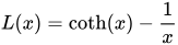
The Langevin function ( $L(x)$ ) was named after Paul Langevin who published two papers with this function in 1905 to describe paramagnetism by statistical mechanics. Written as:

$L(x)=\coth(x)-{\frac {1}{x}}$

It could be derived by describing how magnetic moments are aligned by a magnetic field, considering the statistical thermodynamics. One derivation could be seen here:

Click "show" to see a derivation of this function:
The energy for each magnetic moment will be $E=-\mu H\cos \theta ,$ where $\theta$ is the angle between the magnetic moment and the magnetic field (which we take to be pointing in the $z$ coordinate.) The corresponding partition function is $Z=\int _{0}^{2\pi }d\phi \int _{0}^{\pi }d\theta \sin \theta e^{(\mu H\cos \theta /k_{\text{B}}T)}.$ Here we could simplify to replace $x=\mu H/k_{\text{B}}T$ . We see there is no dependence on the $\phi$ angle, and also we can change variables to $a=\cos \theta$ to obtain $Z=2\pi \int _{-1}^{1}da\cdot e^{xa}=2\pi {\frac {e^{x}-e^{-x}}{x}}={\frac {4\pi \sinh(x)}{x.}}$ Now, the expected value of the $z$ component of the magnetization (the other two are seen to be null (due to integration over $\phi$ ), as they should) will be given by $\left\langle \mu _{z}\right\rangle ={\frac {1}{Z}}\int _{0}^{2\pi }d\phi \int _{0}^{\pi }d\theta \sin \theta \exp(x\cos \theta )\left[\mu \cos \theta \right].$ To simplify the calculation, we see this can be written as a differentiation of $Z$ : $\left\langle \mu _{z}\right\rangle ={\frac {k_{\text{B}}T}{Z}}{\frac {\partial Z}{\partial B}}=k_{\text{B}}T{\frac {\partial \ln Z}{\partial B}}$ Carrying out the derivation we find $M=N\left\langle \mu _{z}\right\rangle =N\mu \cdot L(\mu H/k_{\text{B}}T),$ where $L$ is the Langevin function: $L(x)=\coth x-{\frac {1}{x}}.$

Click "show" to see a derivation of this function:

The energy for each magnetic moment will be

$E=-\mu H\cos \theta ,$

where $\theta$ is the angle between the magnetic moment and the magnetic field (which we take to be pointing in the $z$ coordinate.) The corresponding partition function is

$Z=\int _{0}^{2\pi }d\phi \int _{0}^{\pi }d\theta \sin \theta e^{(\mu H\cos \theta /k_{\text{B}}T)}.$

Here we could simplify to replace $x=\mu H/k_{\text{B}}T$ . We see there is no dependence on the $\phi$ angle, and also we can change variables to $a=\cos \theta$ to obtain

$Z=2\pi \int _{-1}^{1}da\cdot e^{xa}=2\pi {\frac {e^{x}-e^{-x}}{x}}={\frac {4\pi \sinh(x)}{x.}}$

Now, the expected value of the $z$ component of the magnetization (the other two are seen to be null (due to integration over $\phi$ ), as they should) will be given by

$\left\langle \mu _{z}\right\rangle ={\frac {1}{Z}}\int _{0}^{2\pi }d\phi \int _{0}^{\pi }d\theta \sin \theta \exp(x\cos \theta )\left[\mu \cos \theta \right].$

To simplify the calculation, we see this can be written as a differentiation of $Z$ :

$\left\langle \mu _{z}\right\rangle ={\frac {k_{\text{B}}T}{Z}}{\frac {\partial Z}{\partial B}}=k_{\text{B}}T{\frac {\partial \ln Z}{\partial B}}$

Carrying out the derivation we find

$M=N\left\langle \mu _{z}\right\rangle =N\mu \cdot L(\mu H/k_{\text{B}}T),$

where $L$ is the Langevin function:

$L(x)=\coth x-{\frac {1}{x}}.$

The Langevin function can also be derived as the classical limit of the Brillouin function, if the magnetic moments can be continuously aligned in the field and the quantum number $J$ would be able to assume all values ( $J\to \infty$ ). The Brillouin function is then simplified into the Langevin function.

Classical or quantum approach?

Langevin function is often seen as the classical theory of paramagnetism, while the Brillouin function is the quantum theory of paramagnetism. When Langevin published the theory paramagnetism in 1905 it was before the adoption of quantum physics. Meaning that Langevin only used concepts of classical physics.

Niels Bohr showed in his thesis that classical statistical mechanics can not be used to explain paramagnetism, and that quantum theory has to be used. This would later be known as the Bohr-Van Leeuwen theorem. The magnetic moment would later be explained in quantum theory by the Bohr magneton ( $\mu _{\text{B}}$ ), which is used in the Brillouin function.

It could be noted that there is a difference in the approaches of Langevin and Bohr, since Langevin assumes a magnetic polarization $\mu$ as the basis for the derivation, while Bohr start the derivation from motions of electrons and a model of an atom. Langevin is still assuming a fix magnetic dipole. This could be expressed as by J. H. Van Vleck: "When Langevin assumed that the magnetic moment of the atom or molecule had a fixed value $\mu$ , he was quantizing the system without realizing it ". This makes the Langevin function to be in the borderland between classical statistical mechanics and quantum theory (as either semi-classical or semi-quantum).

03Langevin function for electric polarization

The Langevin function could also be used to describe electric polarization, in the specific case when the polarization is explained by orientation of (electrically polarized) dipoles. So that the electric polarization is given by:

$P=P_{s}\cdot L(x)$

but here for an electric dipole moment $p$ and an electric field $E_{L}$ (instead of the magnetic equivalents), that is $x={\frac {pE_{L}}{k_{\text{B}}T}}$

04Simplified functions

For small values of x, the Langevin function can be approximated by a truncation of its Taylor series: $L(x)={\tfrac {1}{3}}x-{\tfrac {1}{45}}x^{3}+{\tfrac {2}{945}}x^{5}-{\tfrac {1}{4725}}x^{7}+\dots$ The first term of this series expansion is equivalent to Curie's law, when writing it as

$L(x)\approx {\frac {x}{3}}$

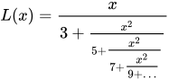
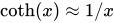
An alternative, better behaved approximation can be derived from the Lambert's continued fraction expansion of tanh(x): $L(x)={\frac {x}{3+{\tfrac {x^{2}}{5+{\tfrac {x^{2}}{7+{\tfrac {x^{2}}{9+\ldots }}}}}}}}$ For small enough x, both approximations are numerically better than a direct evaluation of the actual analytical expression, since the latter suffers from catastrophic cancellation for $x\approx 0$ where $\coth(x)\approx 1/x$ .

Current state-of-the-art diagram of the approximants to the inverse Langevin function,

05Inverse Langevin function

The inverse Langevin function $L^{-1}(x)$ is without an explicit analytical form, but there exist several approximations.

The inverse Langevin function $L^{-1}(x)$ is defined on the open interval (−1, 1). For small values of $x$ , it can be approximated by a truncation of its Taylor series

$L^{-1}(x)=3x+{\tfrac {9}{5}}x^{3}+{\tfrac {297}{175}}x^{5}+{\tfrac {1539}{875}}x^{7}+\dots$

and by the Padé approximant

$L^{-1}(x)=3x{\frac {35-12x^{2}}{35-33x^{2}}}+O(x^{7}).$

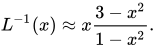
Since this function has no closed form, it is useful to have approximations valid for arbitrary values of $x$ . One popular approximation, valid on the whole range (−1, 1), has been published by A. Cohen: $L^{-1}(x)\approx x{\frac {3-x^{2}}{1-x^{2}}}.$

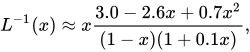
This has a maximum relative error of 4.9% at the vicinity of $x=\pm 0.8$ . Greater accuracy can be achieved by using the formula given by R. Jedynak:

$L^{-1}(x)\approx x{\frac {3.0-2.6x+0.7x^{2}}{(1-x)(1+0.1x)}},$

valid for x ≥ 0. The maximal relative error for this approximation is 1.5% at the vicinity of $x=0.85$ . Even greater accuracy can be achieved by using the formula given by M. Kröger:

$L^{-1}(x)\approx {\frac {3x-x(6x^{2}+x^{4}-2x^{6})/5}{1-x^{2}}}$

The maximal relative error for this approximation is less than 0.28%. More accurate approximation was reported by R. Petrosyan:

$L^{-1}(x)\approx 3x+{\frac {x^{2}}{5}}\sin \left({\frac {7x}{2}}\right)+{\frac {x^{3}}{1-x}},$

valid for x ≥ 0. The maximal relative error for the above formula is less than 0.18%.

New approximation given by R. Jedynak, is the best reported approximant at complexity 11:

$L^{-1}(x)\approx {\frac {x(3-1.00651x^{2}-0.962251x^{4}+1.47353x^{6}-0.48953x^{8})}{(1-x)(1+1.01524x)}},$

valid for x ≥ 0. Its maximum relative error is less than 0.076%.

The current state-of-the-art diagram of the approximants to the inverse Langevin function presents the figure below. It is valid for the rational/Padé approximants,

A recently published paper by R. Jedynak provides a series of the optimal approximants to the inverse Langevin function. The table below reports the results with correct asymptotic behaviors.

Comparison of relative errors for the different optimal rational approximations, which were computed with constraints (Appendix 8 Table 1)

Complexity	Optimal approximation	Maximum relative error [%]
3	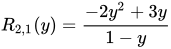$R_{2,1}(y)={\frac {-2y^{2}+3y}{1-y}}$	13
4	$R_{3,1}(y)={\frac {0.88y^{3}-2.88y^{2}+3y}{1-y}}$	0.95
5	$R_{3,2}(y)={\frac {1.1571y^{3}-3.3533y^{2}+3y}{(1-y)(1-0.1962y)}}$	0.56
6	$R_{5,1}(y)={\frac {0.756y^{5}-1.383y^{4}+1.5733y^{3}-2.9463y^{2}+3y}{1-y}}$	0.16
7	$R_{3,4}(y)={\frac {2.14234y^{3}-4.22785y^{2}+3y}{(1-y)\left(0.71716y^{3}-0.41103y^{2}-0.39165y+1\right)}}$	0.082

Also recently, an efficient near-machine precision approximant, based on spline interpolations, has been proposed by Benítez and Montáns, where MATLAB code is also given to generate the spline-based approximant and to compare many of the previously proposed approximants in all the function domain.

Inverse Brillouin function

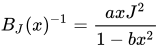
Approximations could also be used to express the inverse Brillouin function ( $B_{J}(x)^{-1}$ ). Takacs proposed the following approximation to the inverse of the Brillouin function: $B_{J}(x)^{-1}={\frac {axJ^{2}}{1-bx^{2}}}$ where the constants $a$ and $b$ are defined to be

$a={\frac {0.5(1+2J)(1-0.055)}{(J-0.27)2J}}+{\frac {0.1}{J^{2}}}$
$b=0.8$

Watch videos about Brillouin and Langevin functionsExplainers and documentaries on YouTube (opens in a new tab)

Sources and credits

This article is adapted from the Wikipedia article “Brillouin and Langevin functions”, written by its contributors and licensed under CC BY-SA 4.0. Fathomly has changed the layout, removed citation markers, navigation and maintenance notices, and adjusted punctuation. This adapted version is shared under the same license. For references, see the original article.

Images, from Wikimedia Commons:

Mplwp Langevin-function tanhx3.svg by Geek3, CC BY 3.0
Cohen and Jedynak approximations.gif by Jedynakr, CC BY-SA 4.0
Approximants to the inverse Langevin function.png by Jedynakr, CC BY-SA 4.0

Fathomly is not affiliated with or endorsed by the Wikimedia Foundation. Spotted a problem? Tell us.