Encyclopedia

Kernel principal component analysis

Multivariate statistical technique

Wikipedia contributorsAdapted for Fathomly · View authors

4 min read
Source updated July 10, 2025

In the field of multivariate statistics, kernel principal component analysis (kernel PCA) is an extension of principal component analysis (PCA) using techniques of kernel methods. Using a kernel, the originally linear operations of PCA are performed in a reproducing kernel Hilbert space.

01Background: Linear PCA

Recall that conventional PCA operates on zero-centered data; that is,

${\frac {1}{N}}\sum _{i=1}^{N}\mathbf {x} _{i}=\mathbf {0}$ ,

where $\mathbf {x} _{i}$ is one of the $N$ multivariate observations. It operates by diagonalizing the covariance matrix,

$C={\frac {1}{N}}\sum _{i=1}^{N}\mathbf {x} _{i}\mathbf {x} _{i}^{\top }$

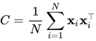
in other words, it gives an eigendecomposition of the covariance matrix:

$\lambda \mathbf {v} =C\mathbf {v}$

which can be rewritten as

$\lambda \mathbf {x} _{i}^{\top }\mathbf {v} =\mathbf {x} _{i}^{\top }C\mathbf {v} \quad {\textrm {for}}~i=1,\ldots ,N$ .

02Introduction of the Kernel to PCA

To understand the utility of kernel PCA, particularly for clustering, observe that, while N points cannot, in general, be linearly separated in $d<N$ dimensions, they can almost always be linearly separated in $d\geq N$ dimensions. That is, given N points, $\mathbf {x} _{i}$ , if we map them to an N-dimensional space with

$\Phi (\mathbf {x} _{i})$ where $\Phi :\mathbb {R} ^{d}\to \mathbb {R} ^{N}$ ,

it is easy to construct a hyperplane that divides the points into arbitrary clusters. Of course, this $\Phi$ creates linearly independent vectors, so there is no covariance on which to perform eigendecomposition explicitly as we would in linear PCA.

Instead, in kernel PCA, a non-trivial, arbitrary $\Phi$ function is 'chosen' that is never calculated explicitly, allowing the possibility to use very-high-dimensional $\Phi$ 's if we never have to actually evaluate the data in that space. Since we generally try to avoid working in the $\Phi$ -space, which we will call the 'feature space', we can create the N-by-N kernel

$K=k(\mathbf {x} ,\mathbf {y} )=(\Phi (\mathbf {x} ),\Phi (\mathbf {y} ))=\Phi (\mathbf {x} )^{T}\Phi (\mathbf {y} )$

which represents the inner product space (see Gramian matrix) of the otherwise intractable feature space. The dual form that arises in the creation of a kernel allows us to mathematically formulate a version of PCA in which we never actually solve the eigenvectors and eigenvalues of the covariance matrix in the $\Phi (\mathbf {x} )$ -space (see Kernel trick). The N-elements in each column of K represent the dot product of one point of the transformed data with respect to all the transformed points (N points). Some well-known kernels are shown in the example below.

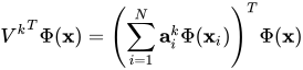
Because we are never working directly in the feature space, the kernel-formulation of PCA is restricted in that it computes not the principal components themselves, but the projections of our data onto those components. To evaluate the projection from a point in the feature space $\Phi (\mathbf {x} )$ onto the kth principal component $V^{k}$ (where superscript k means the component k, not powers of k)

${V^{k}}^{T}\Phi (\mathbf {x} )=\left(\sum _{i=1}^{N}\mathbf {a} _{i}^{k}\Phi (\mathbf {x} _{i})\right)^{T}\Phi (\mathbf {x} )$

We note that $\Phi (\mathbf {x} _{i})^{T}\Phi (\mathbf {x} )$ denotes dot product, which is simply the elements of the kernel $K$ . It seems all that's left is to calculate and normalize the $\mathbf {a} _{i}^{k}$ , which can be done by solving the eigenvector equation

$N\lambda \mathbf {a} =K\mathbf {a}$

where $N$ is the number of data points in the set, and $\lambda$ and $\mathbf {a}$ are the eigenvalues and eigenvectors of $K$ . Then to normalize the eigenvectors $\mathbf {a} ^{k}$ , we require that

$1=(V^{k})^{T}V^{k}$

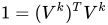
Care must be taken regarding the fact that, whether or not $x$ has zero-mean in its original space, it is not guaranteed to be centered in the feature space (which we never compute explicitly). Since centered data is required to perform an effective principal component analysis, we 'centralize' $K$ to become $K'$

$K'=K-\mathbf {1_{N}} K-K\mathbf {1_{N}} +\mathbf {1_{N}} K\mathbf {1_{N}}$

where $\mathbf {1_{N}}$ denotes a N-by-N matrix for which each element takes value $1/N$ . We use $K'$ to perform the kernel PCA algorithm described above.

One caveat of kernel PCA should be illustrated here. In linear PCA, we can use the eigenvalues to rank the eigenvectors based on how much of the variation of the data is captured by each principal component. This is useful for data dimensionality reduction and it could also be applied to KPCA. However, in practice there are cases that all variations of the data are same. This is typically caused by a wrong choice of kernel scale.

03Large datasets

In practice, a large data set leads to a large K, and storing K may become a problem. One way to deal with this is to perform clustering on the dataset, and populate the kernel with the means of those clusters. Since even this method may yield a relatively large K, it is common to compute only the top P eigenvalues and eigenvectors of the eigenvalues are calculated in this way.

04Example

Consider three concentric clouds of points (shown); we wish to use kernel PCA to identify these groups. The color of the points does not represent information involved in the algorithm, but only shows how the transformation relocates the data points.

First, consider the kernel

$k({\boldsymbol {x}},{\boldsymbol {y}})=({\boldsymbol {x}}^{\mathrm {T} }{\boldsymbol {y}}+1)^{2}$

Applying this to kernel PCA yields the next image.

Now consider a Gaussian kernel:

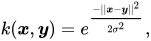
$k({\boldsymbol {x}},{\boldsymbol {y}})=e^{\frac {-||{\boldsymbol {x}}-{\boldsymbol {y}}||^{2}}{2\sigma ^{2}}},$

That is, this kernel is a measure of closeness, equal to 1 when the points coincide and equal to 0 at infinity.

Note in particular that the first principal component is enough to distinguish the three different groups, which is impossible using only linear PCA, because linear PCA operates only in the given (in this case two-dimensional) space, in which these concentric point clouds are not linearly separable.

05Applications

Kernel PCA has been demonstrated to be useful for novelty detection and image de-noising.

Watch videos about Kernel principal component analysisExplainers and documentaries on YouTube (opens in a new tab)

Sources and credits

This article is adapted from the Wikipedia article “Kernel principal component analysis”, written by its contributors and licensed under CC BY-SA 4.0. Fathomly has changed the layout, removed citation markers, navigation and maintenance notices, and adjusted punctuation. This adapted version is shared under the same license. For references, see the original article.

Images, from Wikimedia Commons: