Inverse Gaussian distribution
Family of continuous probability distributions

In probability theory, the inverse Gaussian distribution (also known as the Wald distribution) is a two-parameter family of continuous probability distributions with support on 
Its probability density function is given by

for 


The inverse Gaussian distribution has several properties analogous to a Gaussian distribution. The name can be misleading: it is an inverse only in that, while the Gaussian describes a Brownian motion's level at a fixed time, the inverse Gaussian describes the distribution of the time a Brownian motion with positive drift takes to reach a fixed positive level. The relationship between the Gaussian and inverse Gaussian distributions is thus the same as the relationship between the binomial (number of successes for a fixed number of Bernoulli trials) and negative binomial (number of Bernoulli trials for a fixed number of successes) distributions.
The y-axis reflections of the cumulant generating functions of the Gaussian and inverse Gaussian distributions are inverse of each other (i.e., the graphs of the two cumulant generating functions are reflections of each other across the line 
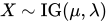
To indicate that a random variable 
01Properties
Single parameter form
The probability density function (pdf) of the inverse Gaussian distribution has a single parameter form given by

In this form, the mean and variance of the distribution are equal, ![\mathbb {E} [X]=\operatorname {Var} (X)](https://wikimedia.org/api/rest_v1/media/math/render/svg/003b66ba3f1961f5f17e77412a85f874583195fa)
Also, the cumulative distribution function (cdf) of the single parameter inverse Gaussian distribution is related to the standard normal distribution by

where 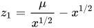


In the single parameter form, the MGF simplifies to
![M(t)=\exp[\mu (1-{\sqrt {1-2t}})].](https://wikimedia.org/api/rest_v1/media/math/render/svg/ae6080ed21f32de632d3783d40b151ec12192381)
An inverse Gaussian distribution in double parameter form 


The above paragraph can be re-written as: if 


The standard form of inverse Gaussian distribution is

Summation
If 



The special case 
Note that
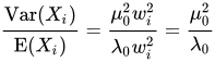
is constant for all 

Scaling
For any 

Exponential family
The inverse Gaussian distribution is a two-parameter exponential family with natural parameters 


For

Indeed, with 
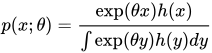
is a density over the reals. Evaluating the integral, we get

Substituting 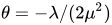

02Relationship with Brownian motion
Let the stochastic process 


where 

Then the first passage time for a fixed level 

i.e

(cf. Schrödinger equation 19, Smoluchowski, equation 8, and Folks, equation 1).
| Derivation of the first passage time distribution |
|---|
|
Suppose that we have a Brownian motion And suppose that we wish to find the probability density function for the time when the process first hits some barrier where Define a point where Now we must determine the value of At Therefore, the full solution to the BVP is: Now that we have the full probability density function, we are ready to find the first passage time distribution where Assuming that |
 defined by:
 - known as the first passage time. The
  is:
is:
 is the
  , which may be solved using the
  , is:
, is:![\varphi (t,x)={1 \over {\sqrt {2\pi \sigma ^{2}t}}}\exp \left[-{(x-x_{0}-\nu t)^{2} \over {2\sigma ^{2}t}}\right]](https://wikimedia.org/api/rest_v1/media/math/render/svg/4cbc3d37009e3df657cf10626e3ac610e886b612)



 is a constant. Due to the linearity of the BVP, the solution to the Fokker-Planck equation with this initial condition is:
![p(t,x)={1 \over {\sqrt {2\pi \sigma ^{2}t}}}\left\{\exp \left[-{(x-x_{0}-\nu t)^{2} \over {2\sigma ^{2}t}}\right]-A\exp \left[-{(x-m-\nu t)^{2} \over {2\sigma ^{2}t}}\right]\right\}](https://wikimedia.org/api/rest_v1/media/math/render/svg/3c6de71603d6b58902d5041f7f411cbe9e89bd1b)




![p(t,x)={1 \over {\sqrt {2\pi \sigma ^{2}t}}}\left\{\exp \left[-{(x-x_{0}-\nu t)^{2} \over {2\sigma ^{2}t}}\right]-e^{2\nu (\alpha -x_{0})/\sigma ^{2}}\exp \left[-{(x+x_{0}-2\alpha -\nu t)^{2} \over {2\sigma ^{2}t}}\right]\right\}](https://wikimedia.org/api/rest_v1/media/math/render/svg/3908c9c70eea2d98524cf0852c7599dc4ab823bd)


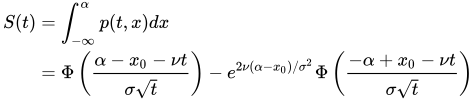
 is the
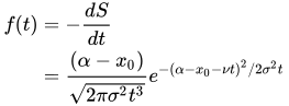
 , the first passage time follows an inverse Gaussian distribution:
![f(t)={\alpha \over {\sqrt {2\pi \sigma ^{2}t^{3}}}}e^{-(\alpha -\nu t)^{2}/2\sigma ^{2}t}\sim {\text{IG}}\left[{\alpha \over {\nu }},\left({\alpha \over {\sigma }}\right)^{2}\right]](https://wikimedia.org/api/rest_v1/media/math/render/svg/e4a067af1e7148d854eabb348d311e4baf500edb)
When drift is zero
A common special case of the above arises when the Brownian motion has no drift. In that case, parameter 

(see also Bachelier). This is a Lévy distribution with parameters 

03Maximum likelihood
The model where

with all 

Solving the likelihood equation yields the following maximum likelihood estimates




04Sampling from an inverse-Gaussian distribution
The following algorithm may be used.
Generate a random variate from a normal distribution with mean
and standard deviation equal
Square the value
and use the relation
Generate another random variate, this time sampled from a uniform distribution between
If
then return
else return





Sample code in Java:
public double inverseGaussian(double mu, double lambda) { Random rand = new Random(); double v = rand.nextGaussian(); // Sample from a normal distribution with a mean of 0 and 1 standard deviation double y = v * v; double x = mu + (mu * mu * y) / (2 * lambda) - (mu / (2 * lambda)) * Math.sqrt(4 * mu * lambda * y + mu * mu * y * y); double test = rand.nextDouble(); // Sample from a uniform distribution between 0 and 1 if (test <= (mu) / (mu + x)) return x; else return (mu * mu) / x; }And to plot Wald distribution in Python using matplotlib and NumPy:
import matplotlib.pyplot as plt import numpy as np h = plt.hist(np.random.wald(3, 2, 100000), bins = 200, density = True) plt.show()
05Related distributions
- If
for any number
.
- If
then
.
- If
then
.
- If
then
.
- If
.
The convolution of an inverse Gaussian distribution (a Wald distribution) and an exponential (an ex-Wald distribution) is used as a model for response times in psychology, with visual search as one example.
06History
This distribution appears to have been first derived in 1900 by Louis Bachelier as the time a stock reaches a certain price for the first time. In 1915 it was used independently by Erwin Schrödinger and Marian v. Smoluchowski as the time to first passage of a Brownian motion. In the field of reproduction modeling it is known as the Hadwiger function, after Hugo Hadwiger who described it in 1940. Abraham Wald re-derived this distribution in 1944 as the limiting form of a sample in a sequential probability ratio test. The name inverse Gaussian was proposed by Maurice Tweedie in 1945. Tweedie investigated this distribution in 1956 and 1957 and established some of its statistical properties. The distribution was extensively reviewed by Folks and Chhikara in 1978.
Rated inverse Gaussian distribution
Assuming that the time intervals between occurrences of a random phenomenon follow an inverse Gaussian distribution, the probability distribution for the number of occurrences of this event within a specified time window is referred to as rated inverse Gaussian. While, first and second moment of this distribution are calculated, the derivation of the moment generating function remains an open problem.
07Numeric computation and software
Despite the simple formula for the probability density function, numerical probability calculations for the inverse Gaussian distribution nevertheless require special care to achieve full machine accuracy in floating point arithmetic for all parameter values. Functions for the inverse Gaussian distribution are provided for the R programming language by several packages including rmutil, SuppDists, STAR, invGauss, LaplacesDemon, and statmod.
Sources and credits
This article is adapted from the Wikipedia article “Inverse Gaussian distribution”, written by its contributors and licensed under CC BY-SA 4.0. Fathomly has changed the layout, removed citation markers, navigation and maintenance notices, and adjusted punctuation. This adapted version is shared under the same license. For references, see the original article.
Images, from Wikimedia Commons:
- Inverse Gaussian Probability Densitiy Function.svg by Gerhard Thallinger, CC BY-SA 4.0
- Inverse gaussian as stopping time of random walk.png by Cosmia Nebula, CC BY-SA 4.0
- Wald Distribution matplotlib.jpg by Bluemix, CC BY-SA 3.0
Fathomly is not affiliated with or endorsed by the Wikimedia Foundation. Spotted a problem? Tell us.
