Encyclopedia

Hyperarithmetical theory

Generalization of Turing computability

Wikipedia contributorsAdapted for Fathomly · View authors

8 min read
Source updated June 25, 2026

In computability theory, hyperarithmetic theory is a generalization of Turing computability. It has close connections with definability in second-order arithmetic and with weak systems of set theory such as Kripke-Platek set theory. It is an important tool in effective descriptive set theory.

The central focus of hyperarithmetic theory is the sets of natural numbers known as hyperarithmetic sets. There are three equivalent ways of defining this class of sets; the study of the relationships between these different definitions is one motivation for the study of hyperarithmetical theory.

01Hyperarithmetical sets and definability

The first definition of the hyperarithmetic sets uses the analytical hierarchy. A set of natural numbers is classified at level $\Sigma _{1}^{1}$ of this hierarchy if it is definable by a formula of second-order arithmetic with only existential set quantifiers and no other set quantifiers. A set is classified at level $\Pi _{1}^{1}$ of the analytical hierarchy if it is definable by a formula of second-order arithmetic with only universal set quantifiers and no other set quantifiers. A set is $\Delta _{1}^{1}$ if it is both $\Sigma _{1}^{1}$ and $\Pi _{1}^{1}$ . The hyperarithmetical sets are exactly the $\Delta _{1}^{1}$ sets.

02Hyperarithmetical sets and iterated Turing jumps: the hyperarithmetical hierarchy

The definition of hyperarithmetical sets as $\Delta _{1}^{1}$ does not directly depend on computability results. A second, equivalent, definition shows that the hyperarithmetical sets can be defined using infinitely iterated Turing jumps. This second definition also shows that the hyperarithmetical sets can be classified into a hierarchy extending the arithmetical hierarchy; the hyperarithmetical sets are exactly the sets that are assigned a rank in this hierarchy.

Each level of the hyperarithmetical hierarchy is indexed by a countable ordinal number (ordinal), but not all countable ordinals correspond to a level of the hierarchy. The ordinals used by the hierarchy are those with an ordinal notation, which is a concrete, effective description of the ordinal.

An ordinal notation is an effective description of a countable ordinal by a natural number. A system of ordinal notations is required in order to define the hyperarithmetic hierarchy. The fundamental property an ordinal notation must have is that it describes the ordinal in terms of smaller ordinals in an effective way. The following inductive definition is typical; it uses a pairing function $\langle \cdot ,\cdot \rangle$ .

The number 0 is a notation for the ordinal 0.
If n is a notation for an ordinal λ then $\langle 1,n\rangle$ is a notation for λ + 1;
Suppose that δ is a limit ordinal. A notation for δ is a number of the form $\langle 2,e\rangle$ , where e is the index of a total computable function $\phi _{e}$ such that for each n, $\phi _{e}(n)$ is a notation for an ordinal λ_n less than δ and δ is the sup of the set $\{\lambda _{n}\mid n\in \mathbb {N} \}$ .

This may also be defined by taking effective joins at all levels instead of only notations for limit ordinals.

There are only countably many ordinal notations, since each notation is a natural number; thus there is a countable ordinal that is the supremum of all ordinals that have a notation. This ordinal is known as the Church-Kleene ordinal and is denoted $\omega _{1}^{CK}$ . Note that this ordinal is still countable, the symbol being only an analogy with the first uncountable ordinal, $\omega _{1}$ . The set of all natural numbers that are ordinal notations is denoted ${\mathcal {O}}$ and called Kleene's ${\mathcal {O}}$ .

Ordinal notations are used to define iterated Turing jumps. The sets of natural numbers used to define the hierarchy are $0^{(\delta )}$ for each $\delta <\omega _{1}^{CK}$ . $0^{(\delta )}$ is sometimes also denoted $H(\delta )$ , or $H_{e}$ for a notation $e$ for $\delta$ . Suppose that δ has notation e. These sets were first defined by Davis (1950) and Mostowski (1951). The set $0^{(\delta )}$ is defined using e as follows.

If δ = 0 then $0^{(\delta )}=0$ is the empty set.
If δ = λ + 1 then $0^{(\delta )}$ is the Turing jump of $0^{(\lambda )}$ . The sets $0^{(1)}$ and $0^{(2)}$ are $0'$ and $0''$ , respectively.
If δ is a limit ordinal, let $\langle \lambda _{n}\mid n\in \mathbb {N} \rangle$ be the sequence of ordinals less than δ given by the notation e. The set $0^{(\delta )}$ is given by the rule $0^{(\delta )}=\{\langle n,i\rangle \mid i\in 0^{(\lambda _{n})}\}$ . This is the effective join of the sets $0^{(\lambda _{n})}$ .

Although the construction of $0^{(\delta )}$ depends on having a fixed notation for δ, and each infinite ordinal has many notations, a theorem of Clifford Spector shows that the Turing degree of $0^{(\delta )}$ depends only on δ, not on the particular notation used, and thus $0^{(\delta )}$ is well defined up to Turing degree.

The hyperarithmetical hierarchy is defined from these iterated Turing jumps. A set X of natural numbers is classified at level δ of the hyperarithmetical hierarchy, for $\delta <\omega _{1}^{CK}$ , if X is Turing reducible to $0^{(\delta )}$ . There will always be a least such δ if there is any; it is this least δ that measures the level of uncomputability of X.

03Hyperarithmetical sets and constructibility

Let $L_{\alpha }$ denote the $\alpha$ th level of the constructible hierarchy, and let $n:{\mathcal {O}}\to \omega _{1}^{CK}$ be the map from a member of Kleene's O to the ordinal it represents. A subset of $\mathbb {N}$ is hyperarithmetical if and only if it is a member of $L_{\omega _{1}^{CK}}$ . A subset of $\mathbb {N}$ is definable by a $\Pi _{1}^{1}$ formula if and only if its image under $n$ is $\Sigma _{1}$ -definable on $L_{\omega _{1}^{CK}}$ , where $\Sigma _{1}$ is from the Lévy hierarchy of formulae.

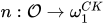
The Spector-Gandy theorem states that a subset $x$ of $\mathbb {N}$ is definable by a $\Pi _{1}^{1}$ formula if and only if there is a $\Sigma _{1}$ formula $\phi (u)$ such that $n\in x$ iff $L_{\omega _{1}^{CK}}\vDash \phi (n)$ . ^{Theorem 3.7.1}

04Hyperarithmetical sets and recursion in higher types

A third characterization of the hyperarithmetical sets, due to Kleene, uses higher-type computable functionals. The type-2 functional ${}^{2}E\colon \mathbb {N} ^{\mathbb {N} }\to \mathbb {N}$ is defined by the following rules:

${}^{2}E(f)=1\quad$ if there is an i such that f(i) > 0,

${}^{2}E(f)=0\quad$ if there is no i such that f(i) > 0.

Using a precise definition of computability relative to a type-2 functional, Kleene showed that a set of natural numbers is hyperarithmetical if and only if it is computable relative to ${}^{2}E$ .

05Example: the truth set of arithmetic

Every arithmetical set is hyperarithmetical, but there are many other hyperarithmetical sets. One example of a hyperarithmetical, nonarithmetical set is the set T of Gödel numbers of formulas of Peano arithmetic that are true in the standard natural numbers $\mathbb {N}$ . The set T is Turing equivalent to the set $0^{(\omega )}$ , and so is not high in the hyperarithmetical hierarchy, although it is not arithmetically definable by Tarski's indefinability theorem.

06Fundamental results

The fundamental results of hyperarithmetic theory show that the three definitions above define the same collection of sets of natural numbers. These equivalences are due to Kleene. Another characterization is given by the Suslin-Kleene theorem.

Completeness results are also fundamental to the theory. A set of natural numbers is $\Pi _{1}^{1}$ complete if it is at level $\Pi _{1}^{1}$ of the analytical hierarchy and every $\Pi _{1}^{1}$ set of natural numbers is many-one reducible to it. The definition of a $\Pi _{1}^{1}$ complete subset of Baire space ( $\mathbb {N} ^{\mathbb {N} }$ ) is similar. Several sets associated with hyperarithmetic theory are $\Pi _{1}^{1}$ complete:

Kleene's ${\mathcal {O}}$ , the set of natural numbers that are notations for ordinal numbers
The set of natural numbers e such that the computable function $\phi _{e}\colon \mathbb {N} ^{2}\to 2$ computes the characteristic function of a well ordering of the natural numbers. These are the indices of recursive ordinals.
The set of elements of Baire space that are the characteristic functions of a well ordering of the natural numbers (using an effective isomorphism $\mathbb {N} ^{\mathbb {N} }\cong \mathbb {N} ^{\mathbb {N} \times \mathbb {N} })$ .

Results known as $\Sigma _{1}^{1}$ bounding follow from these completeness results. For any $\Sigma _{1}^{1}$ set S of ordinal notations, there is an $\alpha <\omega _{1}^{CK}$ such that every element of S is a notation for an ordinal less than $\alpha$ . For any $\Sigma _{1}^{1}$ subset T of Baire space consisting only of characteristic functions of well orderings, there is an $\alpha <\omega _{1}^{CK}$ such that each ordinal represented in T is less than $\alpha$ .

07Relativized hyperarithmeticity and hyperdegrees

The definition of ${\mathcal {O}}$ can be relativized to a set X of natural numbers: in the definition of an ordinal notation, the clause for limit ordinals is changed so that the computable enumeration of a sequence of ordinal notations is allowed to use X as an oracle. The set of numbers that are ordinal notations relative to X is denoted ${\mathcal {O}}^{X}$ . The supremum of ordinals represented in ${\mathcal {O}}^{X}$ is denoted $\omega _{1}^{X}$ ; this is a countable ordinal no smaller than $\omega _{1}^{CK}$ .

The definition of $0^{(\delta )}$ can also be relativized to an arbitrary set $X$ of natural numbers. The only change in the definition is that $X^{(0)}$ is defined to be X rather than the empty set, so that $X^{(1)}=X'$ is the Turing jump of X, and so on. Rather than terminating at $\omega _{1}^{CK}$ the hierarchy relative to X runs through all ordinals less than $\omega _{1}^{X}$ .

The relativized hyperarithmetical hierarchy is used to define hyperarithmetical reducibility. Given sets X and Y, we say $X\leq _{\text{HYP}}Y$ if and only if there is a $\delta <\omega _{1}^{Y}$ such that X is Turing reducible to $Y^{(\delta )}$ . If $X\leq _{\text{HYP}}Y$ and $Y\leq _{\text{HYP}}X$ then the notation $X\equiv _{\text{HYP}}Y$ is used to indicate X and Y are hyperarithmetically equivalent. This is a coarser equivalence relation than Turing equivalence; for example, every set of natural numbers is hyperarithmetically equivalent to its Turing jump but not Turing equivalent to its Turing jump. The equivalence classes of hyperarithmetical equivalence are known as hyperdegrees.

The function that takes a set X to ${\mathcal {O}}^{X}$ is known as the hyperjump by analogy with the Turing jump. Many properties of the hyperjump and hyperdegrees have been established. In particular, it is known that Post's problem for hyperdegrees has a positive answer: for every set X of natural numbers there is a set Y of natural numbers such that $X<_{\text{HYP}}Y<_{\text{HYP}}{\mathcal {O}}^{X}$ .

08Generalizations

Hyperarithmetical theory is generalized by α-recursion theory, which is the study of definable subsets of admissible ordinals. Hyperarithmetical theory is the special case in which α is $\omega _{1}^{CK}$ .

09Relation to other hierarchies

Pointclasses
Lightface		Boldface
Σ⁰ ₀ = Π⁰ ₀ = Δ⁰ ₀ (sometimes the same as Δ⁰ ₁)		Σ⁰ ₀ = Π⁰ ₀ = Δ⁰ ₀ (if defined)
Δ⁰ ₁ = recursive		Δ⁰ ₁ = clopen
Σ⁰ ₁ = recursively enumerable	Π⁰ ₁ = co-recursively enumerable	Σ⁰ ₁ = G = open	Π⁰ ₁ = F = closed
Δ⁰ ₂		Δ⁰ ₂
Σ⁰ ₂	Π⁰ ₂	Σ⁰ ₂ = F_σ	Π⁰ ₂ = G_δ
Δ⁰ ₃		Δ⁰ ₃
Σ⁰ ₃	Π⁰ ₃	Σ⁰ ₃ = G_δσ	Π⁰ ₃ = F_σδ
⋮		⋮
Σ⁰ _<ω = Π⁰ _<ω = Δ⁰ _<ω = Σ¹ ₀ = Π¹ ₀ = Δ¹ ₀ = arithmetical		Σ⁰ _<ω = Π⁰ _<ω = Δ⁰ _<ω = Σ¹ ₀ = Π¹ ₀ = Δ¹ ₀ = boldface arithmetical
⋮		⋮
Δ⁰ _α (α recursive)		Δ⁰ _α (α countable)
Σ⁰ _α	Π⁰ _α	Σ⁰ _α	Π⁰ _α
⋮		⋮
Σ⁰ _ω^CK ₁ = Π⁰ _ω^CK ₁ = Δ⁰ _ω^CK ₁ = Δ¹ ₁ = hyperarithmetical		Σ⁰ _ω₁ = Π⁰ _ω₁ = Δ⁰ _ω₁ = Δ¹ ₁ = B = Borel
Σ¹ ₁ = lightface analytic	Π¹ ₁ = lightface coanalytic	Σ¹ ₁ = A = analytic	Π¹ ₁ = CA = coanalytic
Δ¹ ₂		Δ¹ ₂
Σ¹ ₂	Π¹ ₂	Σ¹ ₂ = PCA	Π¹ ₂ = CPCA
Δ¹ ₃		Δ¹ ₃
Σ¹ ₃	Π¹ ₃	Σ¹ ₃ = PCPCA	Π¹ ₃ = CPCPCA
⋮		⋮
Σ¹ _<ω = Π¹ _<ω = Δ¹ _<ω = Σ² ₀ = Π² ₀ = Δ² ₀ = analytical		Σ¹ _<ω = Π¹ _<ω = Δ¹ _<ω = Σ² ₀ = Π² ₀ = Δ² ₀ = P = projective
⋮		⋮

Watch videos about Hyperarithmetical theoryExplainers and documentaries on YouTube (opens in a new tab)

Sources and credits

This article is adapted from the Wikipedia article “Hyperarithmetical theory”, written by its contributors and licensed under CC BY-SA 4.0. Fathomly has changed the layout, removed citation markers, navigation and maintenance notices, and adjusted punctuation. This adapted version is shared under the same license. For references, see the original article.

Fathomly is not affiliated with or endorsed by the Wikimedia Foundation. Spotted a problem? Tell us.