HHL algorithm
Quantum algorithm for solving systems of linear equations
The Harrow-Hassidim-Lloyd (HHL) algorithm is a quantum algorithm for obtaining certain limited information about the solution to a system of linear equations, introduced by Aram Harrow, Avinatan Hassidim, and Seth Lloyd. Specifically, the algorithm estimates quadratic functions of the solution vector to a given system.
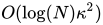
The algorithm is one of the main fundamental algorithms expected to provide a speedup over their classical counterparts, along with Shor's factoring algorithm and Grover's search algorithm. Assuming the system is sparse, has a low condition number 


An implementation of the HHL algorithm was first demonstrated in 2013 by three independent publications, consisting of simple systems on specially designed devices. The first demonstration of a general-purpose version of the algorithm appeared in 2018.
01Overview
Given an 


The algorithm first prepares the quantum state 


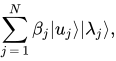
where 

We would then like to apply the linear map taking 

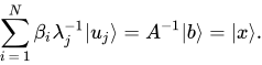
By performing the quantum measurement corresponding to M, we get an estimate of
02Detailed description
Assumptions and initialization
The algorithm requires the following assumptions to hold:
- The algorithm requires A to be Hermitian so that it can be exponentiated into a unitary operator. If A is not Hermitian, one can define a Hermitian matrix
and solve
to obtain
.
- The algorithm requires an efficient procedure to prepare
to
- The algorithm assumes that the state
can be prepared efficiently, where
for some large T. The coefficients of
subroutine described below.
- The algorithm assumes that the unitary operator
.
Uinvert subroutine
The key subroutine to the algorithm, denoted
- Prepare
on register C
- Apply the conditional Hamiltonian evolution (sum)
- Apply the Fourier transform to the register C. Denote the resulting basis states with
for k = 0, ..., T − 1. Define
.
- Adjoin a three-dimensional register S in the state

- Reverse steps 1-3, uncomputing any garbage produced along the way.
The phase estimation procedure in steps 1-3 estimates the eigenvalues of A up to error 
The ancilla register in step 4 is needed to construct a state with inverted eigenvalues corresponding to the diagonalized inverse of A. The states 'nothing', 'well' and 'ill' are used to direct the loop body; 'nothing' indicates that the matrix inversion has not yet taken place, 'well' indicates that it has and the loop should halt, and 'ill' indicates that part of
Main loop
The main loop follows amplitude amplification: starting with 

After each iteration, 


After successfully measuring 'well' on
The quantum measurement corresponding to M then gives an estimate of
03Analysis
Classical efficiency
The best classical algorithm which produces the actual solution vector 

If A is s-sparse and positive semi-definite, then the Conjugate Gradient method can be used to find the solution vector 

When only a summary statistic of the solution vector 
Quantum efficiency
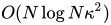
The runtime of the algorithm originally proposed by Harrow et al. was shown to be 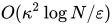





Optimality
The performance of the matrix inversion algorithm depends on the condition number ![[1/\kappa ,1]](https://wikimedia.org/api/rest_v1/media/math/render/svg/c8c84f3742a77e121bb9ef3fda461bfef86128f4)

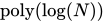
A quantum algorithm for linear systems with poly-logarithmic runtime in
Error analysis
The dominant source of error is the application of 
The phase estimation step errs by 


04Experimental realization
While a general-purpose quantum computer does not yet exist, one can still try to execute a proof of concept implementation of the HHL algorithm. This remained a challenge for years, until three groups independently did so in 2013.
On February 5, 2013, a group led by Stefanie Barz reported an implementation of the HHL algorithm on a photonic quantum computer. The implementation used two consecutive entangling gates on the same pair of polarization-encoded qubits. Two separately controlled NOT gates were realized where the successful operation of the first was heralded by a measurement of two ancillary photons. Experimental measurements of the fidelity in the obtained output state ranged from 64.7% to 98.1% due to the influence of higher-order emissions from spontaneous parametric down-conversion.
On February 8, 2013, Pan et al. reported a proof-of-concept experimental demonstration of the quantum algorithm using a 4-qubit NMR quantum computer. The implementation was tested using linear systems of 2 variables. Across three experiments, the solution vector was obtained with over 96% fidelity.
On February 18, 2013, Cai et al. reported an experimental demonstration solving 2-by-2 linear systems. The quantum circuit was optimized and compiled into a linear optical network with four photonic qubits and four controlled logic gates, which were used to coherently implement the subroutines of the HHL algorithm. For various input vectors, the realization gave solutions with fidelities ranging from 0.825 to 0.993.
Another experimental demonstration using NMR for solving an 8*8 system was reported by Wen et al. in 2018 using the algorithm developed by Subaşı et al.
05Proposed applications
Several concrete applications of the HHL algorithm have been proposed, which analyze the algorithm's input assumptions and output guarantees for particular problems.
- Electromagnetic scattering
- Clader et al. gave a version of the HHL algorithm which allows a preconditioner to be included, which can be used improve the dependence on the condition number. The algorithm was applied to solving for the radar cross-section of a complex shape, which was one of the first examples of an application of the HHL algorithm to a concrete problem.
- Solving linear differential equations
- Berry proposed an algorithm for solving linear, time-dependent initial value problems using the HHL algorithm.
- Solving nonlinear differential equations
- Two groups proposed efficient algorithms for numerically integrating dissipative nonlinear ordinary differential equations. Liu et al. utilized Carleman linearization for second order equations and Lloyd et al. used a mean field linearization method inspired by the nonlinear Schrödinger equation for general order nonlinearities. The resulting linear equations are solved using quantum algorithms for linear differential equations.
- Finite element method
- The finite element method approximates linear partial differential equations using large systems of linear equations. Montanaro and Pallister demonstrate that the HHL algorithm can achieve a polynomial quantum speedup for the resulting linear systems. Exponential speedups are not expected for problems in a fixed dimension or for which the solution meets certain smoothness conditions, such as certain high-order problems in many-body dynamics, or some problems in computational finance.
- Least-squares fitting
- Wiebe et al. gave a quantum algorithm to determine the quality of a least-squares fit. The optimal coefficients cannot be calculated directly from the output of the quantum algorithm, but the algorithm still outputs the optimal least-squares error.
- Machine learning
- Many quantum machine learning algorithms have been developed, a large number of which use the HHL algorithm as a subroutine. The runtime of certain classical algorithms is often polynomial in the size and dimension of a dataset, while the HHL algorithm can give an exponential speedup in some cases. However, a line work initiated by Ewin Tang has found that for most quantum machine learning algorithms, there are classical algorithms giving the same exponential speedups with similar input assumptions.
- Finance
- Proposals for using HHL in finance include solving partial differential equations for the Black-Scholes equation and determining portfolio optimization via a Markowitz solution.
- Quantum chemistry
- The linearized coupled cluster method in quantum chemistry can be recast as a system of linear equations. In 2023, Baskaran et al. proposed the use of HHL algorithm to solve the resulting linear systems. The number of state register qubits in the quantum algorithm is the logarithm of the number of excitations, offering an exponential reduction in the number of required qubits when compared to using the variational quantum eigensolver or quantum phase estimation.
06Implementation difficulties
Recognizing the importance of the HHL algorithm in the field of quantum machine learning, Scott Aaronson analyzes the caveats and factors that could limit the actual quantum advantage of the algorithm.
- the solution vector,
steps the exponential advantage of HHL would vanish.
- the QPE phases calls for the generation of the unitary
- lastly, the vector,
. If actual values of
times, killing the exponential speed-up. However, three ways of avoiding getting the actual values have been proposed: first, if only some properties of the solution are needed; second, if the results are needed only to feed downstream matrix operations; third, if only a sample of the solution is needed.
Sources and credits
This article is adapted from the Wikipedia article “HHL algorithm”, written by its contributors and licensed under CC BY-SA 4.0. Fathomly has changed the layout, removed citation markers, navigation and maintenance notices, and adjusted punctuation. This adapted version is shared under the same license. For references, see the original article.
Fathomly is not affiliated with or endorsed by the Wikimedia Foundation. Spotted a problem? Tell us.