Encyclopedia

Quantum phase estimation algorithm

Quantum algorithm for eigenvalue estimation

Wikipedia contributorsAdapted for Fathomly · View authors

4 min read
Source updated June 8, 2026

In quantum computing, the quantum phase estimation algorithm is a quantum algorithm to estimate the phase corresponding to an eigenvalue of a given unitary operator. Because the eigenvalues of a unitary operator always have unit modulus, they are characterized by their phase, and therefore the algorithm can be equivalently described as retrieving either the phase or the eigenvalue itself. The algorithm was initially introduced by Alexei Kitaev in 1995.

Phase estimation is frequently used as a subroutine in other quantum algorithms, such as Shor's algorithm, the quantum algorithm for linear systems of equations, and the quantum counting algorithm.

01Overview of the algorithm

The algorithm operates on two sets of qubits, referred to in this context as registers. The two registers contain $n$ and $m$ qubits, respectively. Let $U$ be a unitary operator acting on the $m$ -qubit register. The eigenvalues of a unitary operator have unit modulus, and are therefore characterized by their phase. Thus if $|\psi \rangle$ is an eigenvector of $U$ , then $U|\psi \rangle =e^{2\pi i\theta }\left|\psi \right\rangle$ for some $\theta \in \mathbb {R}$ . Due to the periodicity of the complex exponential, we can always assume $0\leq \theta <1$ .

The goal is producing a good approximation for $\theta$ with a small number of gates and a high probability of success. The quantum phase estimation algorithm achieves this assuming oracular access to $U$ , and having $|\psi \rangle$ available as a quantum state. This means that when discussing the efficiency of the algorithm we only worry about the number of times $U$ needs to be used, but not about the cost of implementing $U$ itself.

More precisely, the algorithm returns with high probability an approximation for $\theta$ , within additive error $\varepsilon$ , using $n=O(\log(1/\varepsilon ))$ qubits in the first register, and $O(1/\varepsilon )$ controlled-U operations. Furthermore, we can improve the success probability to $1-\Delta$ for any $\Delta >0$ by using a total of $O(\log(1/\Delta )/\varepsilon )$ uses of controlled-U, and this is optimal.

The circuit for quantum phase estimation.

02Detailed description of the algorithm

State preparation

The initial state of the system is:

$|\Psi _{0}\rangle =|0\rangle ^{\otimes n}|\psi \rangle ,$

where $|\psi \rangle$ is the $m$ -qubit state that evolves through $U$ . We first apply the n-qubit Hadamard gate operation $H^{\otimes n}$ on the first register, which produces the state: $|\Psi _{1}\rangle =(H^{\otimes n}\otimes I_{m})|\Psi _{0}\rangle ={\frac {1}{2^{\frac {n}{2}}}}(|0\rangle +|1\rangle )^{\otimes n}|\psi \rangle ={\frac {1}{2^{n/2}}}\sum _{j=0}^{2^{n}-1}|j\rangle |\psi \rangle .$ Note that here we are switching between binary and $n$ -ary representation for the $n$ -qubit register: the ket $|j\rangle$ on the right-hand side is shorthand for the $n$ -qubit state $|j\rangle \equiv \bigotimes _{\ell =0}^{n-1}|j_{\ell }\rangle$ , where $j=\sum _{\ell =0}^{n-1}j_{\ell }2^{\ell }$ is the binary decomposition of $j$ .

Controlled-U operations

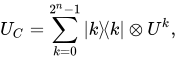
This state $|\Psi _{1}\rangle$ is then evolved through the controlled-unitary evolution $U_{C}$ whose action can be written as $U_{C}(|k\rangle \otimes |\psi \rangle )=|k\rangle \otimes (U^{k}|\psi \rangle ),$ for all $k=0,...,2^{n}-1$ . This evolution can also be written concisely as $U_{C}=\sum _{k=0}^{2^{n}-1}|k\rangle \!\langle k|\otimes U^{k},$ which highlights its controlled nature: it applies $U^{k}$ to the second register conditionally to the first register being $|k\rangle$ . Remembering the eigenvalue condition holding for $|\psi \rangle$ , applying $U_{C}$ to $|\Psi _{1}\rangle$ thus gives $|\Psi _{2}\rangle \equiv U_{C}|\Psi _{1}\rangle =\left({\frac {1}{2^{n/2}}}\sum _{k=0}^{2^{n}-1}e^{2\pi i\theta k}|k\rangle \right)\otimes |\psi \rangle ,$ where we used $U^{k}|\psi \rangle =e^{2\pi ik\theta }|\psi \rangle$ .

To show that $U_{C}$ can also be implemented efficiently, observe that we can write $U_{C}=\prod _{\ell =0}^{n-1}C_{\ell }(U^{2^{\ell }})$ , where $C_{\ell }(U^{2^{\ell }})$ denotes the operation of applying $U^{2^{\ell }}$ to the second register conditionally to the $\ell$ -th qubit of the first register being $|1\rangle$ . Formally, these gates can be characterized by their action as $C_{\ell }(U^{k})(|j\rangle \otimes |\psi \rangle )=|j\rangle \otimes (U^{j_{\ell }k}|\psi \rangle ).$ This equation can be interpreted as saying that the state is left unchanged when $j_{\ell }=0$ , that is, when the $\ell$ -th qubit is $|0\rangle$ , while the gate $U^{k}$ is applied to the second register when the $\ell$ -th qubit is $|1\rangle$ . The composition of these controlled-gates thus gives $\prod _{\ell =0}^{n-1}C_{\ell }(U^{2^{\ell }})(|j\rangle \otimes |\psi \rangle )=|j\rangle \otimes \left(U^{\sum _{\ell =0}^{n-1}j_{\ell }2^{\ell }}|\psi \rangle \right)=U_{C}\left(|j\rangle \otimes |\psi \rangle \right),$ with the last step directly following from the binary decomposition $j=\sum _{\ell =0}^{n-1}j_{\ell }2^{\ell }$ .

From this point onwards, the second register is left untouched, and thus it is convenient to write $|\Psi _{2}\rangle =|{\tilde {\Psi }}_{2}\rangle \otimes |\psi \rangle$ , with $|{\tilde {\Psi }}_{2}\rangle$ the state of the $n$ -qubit register, which is the only one we need to consider for the rest of the algorithm.

Apply inverse quantum Fourier transform

The final part of the circuit involves applying the inverse quantum Fourier transform (QFT) ${\mathcal {QFT}}$ on the first register of $|\Psi _{2}\rangle$ : $|{\tilde {\Psi }}_{3}\rangle ={\mathcal {QFT}}_{2^{n}}^{-1}|{\tilde {\Psi }}_{2}\rangle .$ The QFT and its inverse are characterized by their action on basis states as ${\begin{aligned}{\mathcal {QFT}}_{N}|k\rangle &=N^{-1/2}\sum _{j=0}^{N-1}e^{{\frac {2\pi i}{N}}jk}|j\rangle ,\\{\mathcal {QFT}}_{N}^{-1}|k\rangle &=N^{-1/2}\sum _{j=0}^{N-1}e^{-{\frac {2\pi i}{N}}jk}|j\rangle .\end{aligned}}$ It follows that

$|{\tilde {\Psi }}_{3}\rangle ={\frac {1}{2^{\frac {n}{2}}}}\sum _{k=0}^{2^{n}-1}e^{2\pi i\theta k}\left({\frac {1}{2^{\frac {n}{2}}}}\sum _{x=0}^{2^{n}-1}e^{\frac {-2\pi ikx}{2^{n}}}|x\rangle \right)={\frac {1}{2^{n}}}\sum _{x=0}^{2^{n}-1}\sum _{k=0}^{2^{n}-1}e^{-{\frac {2\pi ik}{2^{n}}}\left(x-2^{n}\theta \right)}|x\rangle .$

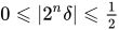
Decomposing the state in the computational basis as ${\textstyle |{\tilde {\Psi }}_{3}\rangle =\sum _{x=0}^{2^{n}-1}c_{x}|x\rangle ,$ the coefficients thus equal $c_{x}\equiv {\frac {1}{2^{n}}}\sum _{k=0}^{2^{n}-1}e^{-{\frac {2\pi ik}{2^{n}}}(x-2^{n}\theta )}={\frac {1}{2^{n}}}\sum _{k=0}^{2^{n}-1}e^{-{\frac {2\pi ik}{2^{n}}}\left(x-a\right)}e^{2\pi i\delta k},$ where we wrote $2^{n}\theta =a+2^{n}\delta ,$ with $a$ is the nearest integer to $2^{n}\theta$ . The difference $2^{n}\delta$ must by definition satisfy $0\leqslant |2^{n}\delta |\leqslant {\tfrac {1}{2}}$ . This amounts to approximating the value of $\theta \in [0,1]$ by rounding $2^{n}\theta$ to the nearest integer.

Measurement

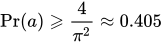
The final step involves performing a measurement in the computational basis on the first register. This yields the outcome $|y\rangle$ with probability $\Pr(y)=|c_{y}|^{2}=\left|{\frac {1}{2^{n}}}\sum _{k=0}^{2^{n}-1}e^{{\frac {-2\pi ik}{2^{n}}}(y-a)}e^{2\pi i\delta k}\right|^{2}.$ It follows that $\operatorname {Pr} (a)=1$ if $\delta =0$ , that is, when $\theta$ can be written as $\theta =a/2^{n}$ , one always finds the outcome $y=a$ . On the other hand, if $\delta \neq 0$ , the probability reads $\operatorname {Pr} (a)={\frac {1}{2^{2n}}}\left|\sum _{k=0}^{2^{n}-1}e^{2\pi i\delta k}\right|^{2}={\frac {1}{2^{2n}}}\left|{\frac {1-{e^{2\pi i2^{n}\delta }}}{1-{e^{2\pi i\delta }}}}\right|^{2}.$ From this expression we can see that $\Pr(a)\geqslant {\frac {4}{\pi ^{2}}}\approx 0.405$ when $\delta \neq 0$ . To see this, we observe that from the definition of $\delta$ we have the inequality $|\delta |\leqslant {\tfrac {1}{2^{n+1}}}$ , and thus: ${\begin{aligned}\Pr(a)&={\frac {1}{2^{2n}}}\left|{\frac {1-{e^{2\pi i2^{n}\delta }}}{1-{e^{2\pi i\delta }}}}\right|^{2}&&{\text{for }}\delta \neq 0\\&={\frac {1}{2^{2n}}}\left|{\frac {2\sin \left(\pi 2^{n}\delta \right)}{2\sin(\pi \delta )}}\right|^{2}&&\left|1-e^{2ix}\right|^{2}=4\left|\sin(x)\right|^{2}\\&={\frac {1}{2^{2n}}}{\frac {\left|\sin \left(\pi 2^{n}\delta \right)\right|^{2}}{|\sin(\pi \delta )|^{2}}}\\&\geqslant {\frac {1}{2^{2n}}}{\frac {\left|\sin \left(\pi 2^{n}\delta \right)\right|^{2}}{|\pi \delta |^{2}}}&&|\sin(\pi \delta )|\leqslant |\pi \delta |\\&\geqslant {\frac {1}{2^{2n}}}{\frac {|2\cdot 2^{n}\delta |^{2}}{|\pi \delta |^{2}}}&&|2\cdot 2^{n}\delta |\leqslant |\sin(\pi 2^{n}\delta )|{\text{ for }}|\delta |\leqslant {\frac {1}{2^{n+1}}}\\&\geqslant {\frac {4}{\pi ^{2}}}.\end{aligned}}$

We conclude that the algorithm provides the best $n$ -bit estimate (i.e., one that is within $1/2^{n}$ of the correct answer) of $\theta$ with probability at least $4/\pi ^{2}$ . By adding a number of extra qubits on the order of $O(\log(1/\epsilon ))$ and truncating the extra qubits the probability can increase to $1-\epsilon$ .

03Toy examples

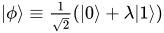
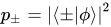
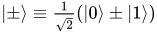
Consider the simplest possible instance of the algorithm, where only $n=1$ qubit, on top of the qubits required to encode $|\psi \rangle$ , is involved. Suppose the eigenvalue of $|\psi \rangle$ reads $\lambda =e^{2\pi i\theta }$ , $\theta \in [0,1)$ . The first part of the algorithm generates the one-qubit state ${\textstyle |\phi \rangle \equiv {\frac {1}{\sqrt {2}}}(|0\rangle +\lambda |1\rangle )$ . Applying the inverse QFT amounts in this case to applying a Hadamard gate. The final outcome probabilities are thus $p_{\pm }=|\langle \pm |\phi \rangle |^{2}$ where ${\textstyle |\pm \rangle \equiv {\frac {1}{\sqrt {2}}}(|0\rangle \pm |1\rangle )$ , or more explicitly, $p_{\pm }={\frac {|1\pm \lambda |^{2}}{4}}={\frac {1\pm \cos(2\pi \theta )}{2}}.$ Suppose $\lambda =1$ , meaning $|\phi \rangle =|+\rangle$ . Then $p_{+}=1$ , $p_{-}=0$ , and we recover deterministically the precise value of $\lambda$ from the measurement outcomes. The same applies if $\lambda =-1$ .

If on the other hand $\lambda =e^{2\pi i/3}$ , then $p_{\pm }=[1\pm \cos(2\pi /3)]/2$ , that is, $p_{+}=1/4$ and $p_{-}=3/4$ . In this case the result is not deterministic, but we still find the outcome $|-\rangle$ as more likely, compatibly with the fact that $2/3$ is closer to 1 than to 0.

More generally, if $\lambda =e^{2\pi i\theta }$ , then $p_{+}\geq 1/2$ if and only if $|\theta |\leq 1/4$ . This is consistent with the results above because in the cases $\lambda =\pm 1$ , corresponding to $\theta =0,1/2$ , the phase is retrieved deterministically, and the other phases are retrieved with higher accuracy the closer they are to these two.

Watch videos about Quantum phase estimation algorithmExplainers and documentaries on YouTube (opens in a new tab)

Sources and credits

This article is adapted from the Wikipedia article “Quantum phase estimation algorithm”, written by its contributors and licensed under CC BY-SA 4.0. Fathomly has changed the layout, removed citation markers, navigation and maintenance notices, and adjusted punctuation. This adapted version is shared under the same license. For references, see the original article.

Images, from Wikimedia Commons:

PhaseCircuit.svg by Omrika, CC BY-SA 4.0

Fathomly is not affiliated with or endorsed by the Wikimedia Foundation. Spotted a problem? Tell us.

Quantum phase estimation algorithm

01Overview of the algorithm

02Detailed description of the algorithm

State preparation

Controlled-U operations

Apply inverse quantum Fourier transform

Measurement

03Toy examples

Sources and credits

Related topics

Shor's algorithm

Quantum counting algorithm

Parity measurement