Encyclopedia

Gabor transform

Special case of the short-time Fourier transform

Wikipedia contributorsAdapted for Fathomly · View authors

4 min read
Source updated July 2, 2025

The Gabor transform, named after Dennis Gabor, is a special case of the short-time Fourier transform. It is used to determine the sinusoidal frequency and phase content of local sections of a signal as it changes over time. The function to be transformed is first multiplied by a Gaussian function, which can be regarded as a window function, and the resulting function is then transformed with a Fourier transform to derive the time-frequency analysis. The window function means that the signal near the time being analyzed will have higher weight. The Gabor transform of a signal x(t) is defined by this formula:

$G_{x}(\tau ,\omega )=\int _{-\infty }^{\infty }x(t)e^{-\pi (t-\tau )^{2}}e^{-j\omega t}\,dt$

The Gaussian function has infinite range and it is impractical for implementation. However, a level of significance can be chosen (for instance 0.00001) for the distribution of the Gaussian function.

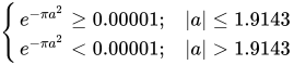
${\begin{cases}e^{-{\pi }a^{2}}\geq 0.00001;&\left|a\right|\leq 1.9143\\e^{-{\pi }a^{2}}<0.00001;&\left|a\right|>1.9143\end{cases}}$

Outside these limits of integration ( $\left|a\right|>1.9143$ ) the Gaussian function is small enough to be ignored. Thus the Gabor transform can be satisfactorily approximated as

$G_{x}(\tau ,\omega )=\int _{-1.9143+\tau }^{1.9143+\tau }x(t)e^{-\pi (t-\tau )^{2}}e^{-j\omega t}\,dt$

This simplification makes the Gabor transform practical and realizable.

The window function width can also be varied to optimize the time-frequency resolution tradeoff for a particular application by replacing the ${-{\pi }(t-\tau )^{2}}$ with ${-{\pi }\alpha (t-\tau )^{2}}$ for some chosen $\alpha$ .

01Inverse Gabor transform

The Gabor transform is invertible. Because it is over-complete, the original signal can be recovered in a variety of ways. For example, the "unwindowing" approach can be used for any 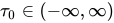$\tau _{0}\in (-\infty ,\infty )$ :

$x(t)=e^{\pi (t-\tau _{0})^{2}}{\frac {1}{2\pi }}\int _{-\infty }^{\infty }G_{x}(\tau _{0},\omega )e^{j\omega t}\,d\omega$

Alternatively, all of the time components can be combined:

$x(t)=\int _{-\infty }^{\infty }{\frac {1}{2\pi }}\int _{-\infty }^{\infty }G_{x}(\tau ,\omega )e^{j\omega t}\,d\omega \,d\tau$

02Properties of the Gabor transform

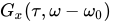
The Gabor transform has many properties like those of the Fourier transform. These properties are listed in the following tables.

	Signal	Gabor transform	Remarks
	$x(t)\,$	$G_{x}(\tau ,\omega )=\int _{-\infty }^{\infty }x(t)e^{-\pi (t-\tau )^{2}}e^{-j\omega t}\,dt$
1	$a\cdot x(t)+b\cdot y(t)\,$	$a\cdot G_{x}(\tau ,\omega )+b\cdot G_{y}(\tau ,\omega )\,$	Linearity property
2	$x(t-t_{0})\,$	$G_{x}(\tau -t_{0},\omega )e^{-j\omega t_{0}}\,$	Shifting property
3	$x(t)e^{j\omega _{0}t}\,$	$G_{x}(\tau ,\omega -\omega _{0})\,$	Modulation property

		Remarks
1	$\int _{-\infty }^{\infty }\left\|G_{x}(\tau ,\omega )\right\|^{2}\,d\omega =\int _{-\infty }^{\infty }\left\|x(t)\right\|^{2}e^{-2\pi (t-\tau )^{2}}dt\approx \int _{\tau -1.9143}^{\tau +1.9143}\left\|x(t)\right\|^{2}e^{-2\pi (t-\tau )^{2}}dt$	Power integration property
2	$\int _{-\infty }^{\infty }\int _{-\infty }^{\infty }G_{x}(\tau ,\omega )G_{y}^{}(\tau ,\omega )\,d\omega \,d\tau =\int _{-\infty }^{\infty }x(t)y^{}(t)\,d\tau$	Energy sum property
3	${\begin{cases}\displaystyle \int _{-\infty }^{\infty }\left\|G_{x}(\tau ,\omega )\right\|^{2}d\omega <e^{-2\pi (t-t_{0})^{2}}\int _{-\infty }^{\infty }\left\|G_{x}(\tau _{0},\omega )\right\|^{2}\,d\omega ;&{\text{if }}x(t)=0{\text{ for }}t>t_{0}\\[12pt]\displaystyle \int _{-\infty }^{\infty }\left\|G_{x}(\tau ,\omega )\right\|^{2}\,d\tau <e^{-(\omega -\omega _{0})^{2}}\int _{-\infty }^{\infty }\left\|G_{x}(\tau ,\omega _{0})\right\|^{2}\,d\tau ;&{\text{if }}X(\omega )=FT[x(t)]=0{\text{ for }}\omega >\omega _{0}\end{cases}}$	Power decay property
4	$\int _{-\infty }^{\infty }G_{x}(\tau ,\omega )e^{j\omega t}\,d\omega =2\pi e^{-\pi \tau ^{2}}x(0)$	Recovery property

03Application and example

The main application of the Gabor transform is used in time-frequency analysis. Take the following function as an example. The input signal has 1 Hz frequency component when t ≤ 0 and has 2 Hz frequency component when t > 0

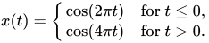
$x(t)={\begin{cases}\cos(2\pi t)&{\text{for }}t\leq 0,\\\cos(4\pi t)&{\text{for }}t>0.\end{cases}}$

But if the total bandwidth available is 5 Hz, other frequency bands except x(t) are wasted. Through time-frequency analysis by applying the Gabor transform, the available bandwidth can be known and those frequency bands can be used for other applications and bandwidth is saved. The right side picture shows the input signal x(t) and the output of the Gabor transform. As was our expectation, the frequency distribution can be separated into two parts. One is t ≤ 0 and the other is t > 0. The white part is the frequency band occupied by x(t) and the black part is not used. Note that for each point in time there is both a negative (upper white part) and a positive (lower white part) frequency component.

04Discrete Gabor-transformation

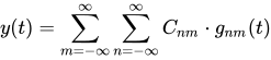
A discrete version of Gabor representation

$y(t)=\sum _{m=-\infty }^{\infty }\sum _{n=-\infty }^{\infty }C_{nm}\cdot g_{nm}(t)$

with $g_{nm}(t)=s(t-m\tau _{0})\cdot e^{j\Omega nt}$

can be derived easily by discretizing the Gabor-basis-function in these equations. Hereby the continuous parameter t is replaced by the discrete time k. Furthermore, the now finite summation limit in Gabor representation has to be considered. In this way, the sampled signal y(k) is split into M time frames of length N. According to $\Omega \leq {\tfrac {2\pi }{\tau _{0}}}$ , the factor Ω for critical sampling is $\Omega ={\tfrac {2\pi }{N}}$ .

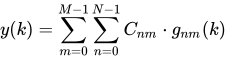
Similar to the DFT (discrete Fourier transformation) a frequency domain split into N discrete partitions is obtained. An inverse transformation of these N spectral partitions then leads to N values y(k) for the time window, which consists of N sample values. For overall M time windows with N sample values, each signal y(k) contains K = N $\cdot$ M sample values: (the discrete Gabor representation)

$y(k)=\sum _{m=0}^{M-1}\sum _{n=0}^{N-1}C_{nm}\cdot g_{nm}(k)$

with $g_{nm}(k)=s(k-mN)\cdot e^{j\Omega nk}$

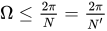
According to the equation above, the N $\cdot$ M coefficients $C_{nm}$ correspond to the number of sample values K of the signal.

For over-sampling $\Omega$ is set to $\Omega \leq {\tfrac {2\pi }{N}}={\tfrac {2\pi }{N^{\prime }}}$ with N′ > N, which results in N′ > N summation coefficients in the second sum of the discrete Gabor representation. In this case, the number of obtained Gabor-coefficients would be M $\cdot$ N′ > K. Hence, more coefficients than sample values are available and therefore a redundant representation would be achieved.

05Scaled Gabor transform

As in short time Fourier transform, the resolution in time and frequency domain can be adjusted by choosing different window function width. In Gabor transform cases, by adding variance $\sigma$ , as following equation:

The scaled (normalized) Gaussian window denotes as:

$W_{\text{gaussian}}(t)=e^{-\sigma \pi t^{2}}$

So the Scaled Gabor transform can be written as:

$G_{x}(t,f)={\sqrt[{4}]{\sigma }}\textstyle \int _{-\infty }^{\infty }\displaystyle e^{-\sigma \pi (\tau -t)^{2}}e^{-j2\pi f\tau }x(\tau )d\tau \qquad$

With a large $\sigma$ , the window function will be narrow, causing higher resolution in time domain but lower resolution in frequency domain. Similarly, a small $\sigma$ will lead to a wide window, with higher resolution in frequency domain but lower resolution in time domain.

06Time-causal analogue of the Gabor transform

When processing temporal signals, data from the future cannot be accessed, which leads to problems if attempting to use Gabor functions for processing real-time signals. A time-causal analogue of the Gabor filter has been developed in based on replacing the Gaussian kernel in the Gabor function with a time-causal and time-recursive kernel referred to as the time-causal limit kernel. In this way, time-frequency analysis based on the resulting complex-valued extension of the time-causal limit kernel makes it possible to capture essentially similar transformations of a temporal signal as the Gabor function can, and corresponding to the Heisenberg group, see for further details.

Watch videos about Gabor transformExplainers and documentaries on YouTube (opens in a new tab)

Sources and credits

This article is adapted from the Wikipedia article “Gabor transform”, written by its contributors and licensed under CC BY-SA 4.0. Fathomly has changed the layout, removed citation markers, navigation and maintenance notices, and adjusted punctuation. This adapted version is shared under the same license. For references, see the original article.

Images, from Wikimedia Commons:

Mplwp gaussian.svg by Geek3, CC BY 3.0
Gabor por stevencys.jpg by Stevencys at English Wikipedia, CC BY-SA 3.0

Fathomly is not affiliated with or endorsed by the Wikimedia Foundation. Spotted a problem? Tell us.

Gabor transform

01Inverse Gabor transform

02Properties of the Gabor transform

03Application and example

04Discrete Gabor-transformation

05Scaled Gabor transform

06Time-causal analogue of the Gabor transform

Sources and credits

Related topics

Gabor filter

Gabor wavelet

Gabor atom