Forney algorithm

Need to introduce terminology and the setup...

Code words look like polynomials. By design, the generator polynomial has consecutive roots α^c, α^c+1, ..., α^c+d−2.

Syndromes

Error location polynomial

The zeros of Λ(x) are X₁⁻¹, ..., X_ν⁻¹. The zeros are the reciprocals of the error locations .

Once the error locations are known, the next step is to determine the error values at those locations. The error values are then used to correct the received values at those locations to recover the original codeword.

In the more general case, the error weights e_j can be determined by solving the linear system

However, there is a more efficient method known as the Forney algorithm, which is based on Lagrange interpolation. First calculate the error evaluator polynomial

Where S(x) is the partial syndrome polynomial:

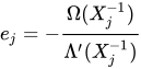
Then evaluate the error values:

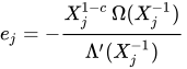
The value c is often called the "first consecutive root" or "fcr". Some codes select c = 1, so the expression simplifies to:

Λ'(x) is the formal derivative of the error locator polynomial Λ(x):

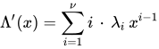
In the above expression, note that i is an integer, and λ_i would be an element of the finite field. The operator ⋅ represents ordinary multiplication (repeated addition in the finite field) which is the same as the finite field's multiplication operator, i.e.

For instance, in characteristic 2, according as i is even or odd.

Lagrange interpolation

Gill (n.d., pp. 52-54) gives a derivation of the Forney algorithm.

Define the erasure locator polynomial

Where the erasure locations are given by j_i. Apply the procedure described above, substituting Γ for Λ.

If both errors and erasures are present, use the error-and-erasure locator polynomial