Final value theorem
Relation between frequency- and time-domain behavior at large time
In mathematical analysis, the final value theorem (FVT) is one of several similar theorems used to relate frequency domain expressions to the time domain behavior as time approaches infinity.
Mathematically, if 


![f[k]](https://wikimedia.org/api/rest_v1/media/math/render/svg/c0c2cac4f7a962e0e8b6e35a6ddb99c8b39763fb)

![\lim _{k\,\to \,\infty }f[k]=\lim _{z\,\to \,1}{(z-1)F(z)}.](https://wikimedia.org/api/rest_v1/media/math/render/svg/99e17af23b8f18ac7e030c383a4996c2c63842ab)
An Abelian final value theorem makes assumptions about the time-domain behavior of ![f(t){\text{ (or }}f[k])](https://wikimedia.org/api/rest_v1/media/math/render/svg/73802d4af59c32b3791abb6e0e0c8a33b9688cad)


![{\text{(or }}\lim _{k\to \infty }f[k])](https://wikimedia.org/api/rest_v1/media/math/render/svg/902dd5ff84f23e22ae19d1437f928aaa5068d807)
01Final value theorems for the Laplace transform
Deducing limt → ∞ f(t)
In the following statements, the notation 


Standard Final Value Theorem
Suppose that every pole of

Final Value Theorem using Laplace transform of the derivative
Suppose that 


Remark
Both limits must exist for the theorem to hold. For example, if 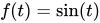

Improved Tauberian converse Final Value Theorem
Suppose that 





Extended Final Value Theorem
Suppose that 
as
and
as
as
as
as

In particular, if 

Generalized Final Value Theorem
Suppose that 


where 
Applications
Final value theorems for obtaining
Deducing lims → 0 s F(s)
Abelian Final Value Theorem
Suppose that 


Elementary proof
Suppose for convenience that 

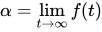


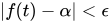


hence

Now for every

On the other hand, since 


Final Value Theorem using Laplace transform of the derivative
Suppose that all of the following conditions are satisfied:
and
have a Laplace transform
is finite
Then

Remark
The proof uses the dominated convergence theorem.
Final Value Theorem for the mean of a function
Let
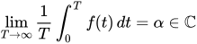
Then

Final Value Theorem for asymptotic sums of periodic functions
Suppose that 


where 


Final Value Theorem for a function that diverges to infinity
Let 
has a Laplace transform for all non-negative integers


Let 

Final Value Theorem for improperly integrable functions (Abel's theorem for integrals)
Let 


To see this, notice that 

![s\int _{0}^{\infty }e^{-st}f(t)\,\mathrm {d} t={\Big [}-e^{-st}f(t){\Big ]}_{t=o}^{\infty }+\int _{0}^{\infty }e^{-st}f'(t)\,\mathrm {d} t=\int _{0}^{\infty }e^{-st}h(t)\,\mathrm {d} t.](https://wikimedia.org/api/rest_v1/media/math/render/svg/1902412d0483ebe75db1e0ca05af285d766313d9)
By the final value theorem, the left-hand side converges to 

To establish the convergence of the improper integral
Applications
Final value theorems for obtaining 


![E[X^{n}]=(-1)^{n}\left.{\frac {d^{n}\rho (s)}{ds^{n}}}\right|_{s=0}.](https://wikimedia.org/api/rest_v1/media/math/render/svg/2edf9220e16e8e0f2fb1cb4d03b905d946cfdb57)







and hence ![E[X^{n}]](https://wikimedia.org/api/rest_v1/media/math/render/svg/20e9c64670d7e2ee2012bcc89f130e0e96fe7bb9)
Examples
Example where FVT holds
For example, for a system described by transfer function
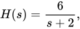
the impulse response converges to
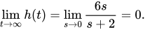
That is, the system returns to zero after being disturbed by a short impulse. However, the Laplace transform of the unit step response is
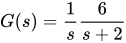
and so the step response converges to

So a zero-state system will follow an exponential rise to a final value of 3.
Example where FVT does not hold
For a system described by the transfer function
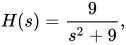
the final value theorem appears to predict the final value of the impulse response to be 0 and the final value of the step response to be 1. However, neither time-domain limit exists, and so the final value theorem predictions are not valid. In fact, both the impulse response and step response oscillate, and (in this special case) the final value theorem describes the average values around which the responses oscillate.
There are two checks performed in Control theory which confirm valid results for the Final Value Theorem:
- All non-zero roots of the denominator of
must have negative real parts.
Rule 1 was not satisfied in this example, in that the roots of the denominator are 

02Final value theorems for the Z transform
Deducing limk → ∞ f[k]
Final Value Theorem
If ![\lim _{k\to \infty }f[k]](https://wikimedia.org/api/rest_v1/media/math/render/svg/939d92a4b7eb4101a84900dcb9ede04a340241f7)
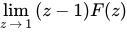
![\lim _{k\to \infty }f[k]=\lim _{z\,\to \,1}{(z-1)F(z)}.](https://wikimedia.org/api/rest_v1/media/math/render/svg/b05faaa5c64654fb3dda2276b4c43248280349ab)
03Final value of linear systems
Continuous-time LTI systems
Final value of the system

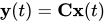
in response to a step input 


Sampled-data systems
The sampled-data system of the above continuous-time LTI system at the aperiodic sampling times 


where 
,

The final value of this system in response to a step input
Sources and credits
This article is adapted from the Wikipedia article “Final value theorem”, written by its contributors and licensed under CC BY-SA 4.0. Fathomly has changed the layout, removed citation markers, navigation and maintenance notices, and adjusted punctuation. This adapted version is shared under the same license. For references, see the original article.
Fathomly is not affiliated with or endorsed by the Wikimedia Foundation. Spotted a problem? Tell us.