Encyclopedia

Expenditure function

Wikipedia contributorsAdapted for Fathomly · View authors

2 min read
Source updated October 21, 2025

In microeconomics, the expenditure function represents the minimum amount of expenditure needed to achieve a given level of utility, given a utility function and the prices of goods.

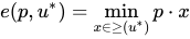
Formally, if there is a utility function $u$ that describes preferences over n goods, the expenditure function $e(p,u^{*})$ is defined as:

$e(p,u^{*})=\min _{x\in \geq (u^{*})}p\cdot x$

where $p$ is the price vector $u^{*}$ is the desired utility level, $\geq (u^{*})=\{x\in {\textbf {R}}_{+}^{n}:u(x)\geq u^{*}\}$ is the set of providing at least utility $u^{*}$ .

Expressed equivalently, the individual minimizes expenditure $x_{1}p_{1}+\dots +x_{n}p_{n}$ subject to the minimal utility constraint that $u(x_{1},\dots ,x_{n})\geq u^{*},$ giving optimal quantities to consume of the various goods as $x_{1}^{*},\dots x_{n}^{*}$ as function of $u^{*}$ and the prices; then the expenditure function is

$e(p_{1},\dots ,p_{n};u^{*})=p_{1}x_{1}^{*}+\dots +p_{n}x_{n}^{*}.$

01Properties

Suppose $u$ is a continuous utility function representing a locally non-satiated preference relation on ${\textbf {R}}_{+}^{n}$ . Then $e(p,u^{*})$ is

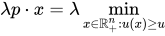
Homogeneous of degree one in p: for all and $\lambda >0$ , $e(\lambda p,u)=\lambda e(p,u);$
Continuous in $p$ and $u;$
Nondecreasing in $p$ and strictly increasing in $u$ provided $p\gg 0;$
Concave in $p$
If the utility function is strictly quasi-concave, there is Shephard's lemma

Proofs

(1) As in the above proposition, note that

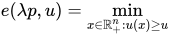
$e(\lambda p,u)=\min _{x\in \mathbb {R} _{+}^{n}:u(x)\geq u}$ $\lambda p\cdot x=\lambda \min _{x\in \mathbb {R} _{+}^{n}:u(x)\geq u}$ $p\cdot x=\lambda e(p,u)$

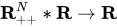
(2) Continue on the domain $e$ : ${\textbf {R}}_{++}^{N}*{\textbf {R}}\rightarrow {\textbf {R}}$

(3) Let $p^{\prime }>p$ and suppose $x\in h(p^{\prime },u)$ . Then $u(h)\geq u$ , and $e(p^{\prime },u)=p^{\prime }\cdot x\geq p\cdot x$ . It follows immediately that $e(p,u)\leq e(p^{\prime },u)$ .

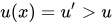
For the second statement, suppose to the contrary that for some $u^{\prime }>u$ , $e(p,u^{\prime })\leq e(p,u)$ Than, for some $x\in h(p,u)$ , $u(x)=u^{\prime }>u$ , which contradicts the "no excess utility" conclusion of the previous proposition

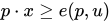
(4) Let $t\in (0,1)$ and suppose $x\in h(tp+(1-t)p^{\prime })$ . Then, $p\cdot x\geq e(p,u)$ and $p^{\prime }\cdot x\geq e(p^{\prime },u)$ , so $e(tp+(1-t)p^{\prime },u)=(tp+(1-t)p^{\prime })\cdot x\geq$ $te(p,u)+(1-t)e(p^{\prime },u)$ .

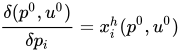
(5) ${\frac {\delta (p^{0},u^{0})}{\delta p_{i}}}=x_{i}^{h}(p^{0},u^{0})$

02Expenditure and indirect utility

The expenditure function is the inverse of the indirect utility function when the prices are kept constant. I.e, for every price vector $p$ and income level $I$ :

$e(p,v(p,I))\equiv I$

There is a duality relationship between the expenditure function and the utility function. If given a specific regular quasi-concave utility function, the corresponding price is homogeneous, and the utility is monotonically increasing expenditure function, conversely, the given price is homogeneous, and the utility is monotonically increasing expenditure function will generate the regular quasi-concave utility function. In addition to the property that prices are once homogeneous and utility is monotonically increasing, the expenditure function usually assumes

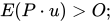
Is a non-negative function, i.e., $E(P\cdot u)>O;$
For P, it is non-decreasing, i.e., $E(p^{1}u)>E(p^{2}u),u>Op^{l}>p^{2}>O_{N}$ ;
E(Pu) is a concave function. That is, $e(np^{l}+(1-n)p^{2})u)>\lambda E(p^{1}u)(1-n)E(p^{2}u)y>0$ $O<\lambda <1p^{l}\geq O_{N}p^{2}\geq O_{N}$

Expenditure function is an important theoretical method to study consumer behavior. Expenditure function is very similar to cost function in production theory. Dual to the utility maximization problem is the cost minimization problem

03Example

Suppose the utility function is the Cobb-Douglas function $u(x_{1},x_{2})=x_{1}^{.6}x_{2}^{.4},$ which generates the demand functions

$x_{1}(p_{1},p_{2},I)={\frac {.6I}{p_{1}}}\;\;\;\;{\rm {and}}\;\;\;x_{2}(p_{1},p_{2},I)={\frac {.4I}{p_{2}}},$

where $I$ is the consumer's income. One way to find the expenditure function is to first find the indirect utility function and then invert it. The indirect utility function $v(p_{1},p_{2},I)$ is found by replacing the quantities in the utility function with the demand functions thus:

$v(p_{1},p_{2},I)=u(x_{1}^{*},x_{2}^{*})=(x_{1}^{*})^{.6}(x_{2}^{*})^{.4}=\left({\frac {.6I}{p_{1}}}\right)^{.6}\left({\frac {.4I}{p_{2}}}\right)^{.4}=(.6^{.6}\times .4^{.4})I^{.6+.4}p_{1}^{-.6}p_{2}^{-.4}=Kp_{1}^{-.6}p_{2}^{-.4}I,$

where $K=(.6^{.6}\times .4^{.4}).$ Then since $e(p_{1},p_{2},u)=e(p_{1},p_{2},v(p_{1},p_{2},I))=I$ when the consumer optimizes, we can invert the indirect utility function to find the expenditure function:

$e(p_{1},p_{2},u)=(1/K)p_{1}^{.6}p_{2}^{.4}u,$

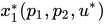
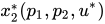
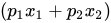
Alternatively, the expenditure function can be found by solving the problem of minimizing $(p_{1}x_{1}+p_{2}x_{2})$ subject to the constraint $u(x_{1},x_{2})\geq u^{*}.$ This yields conditional demand functions $x_{1}^{*}(p_{1},p_{2},u^{*})$ and $x_{2}^{*}(p_{1},p_{2},u^{*})$ and the expenditure function is then

$e(p_{1},p_{2},u^{*})=p_{1}x_{1}^{*}+p_{2}x_{2}^{*}$

Watch videos about Expenditure functionExplainers and documentaries on YouTube (opens in a new tab)

Sources and credits

This article is adapted from the Wikipedia article “Expenditure function”, written by its contributors and licensed under CC BY-SA 4.0. Fathomly has changed the layout, removed citation markers, navigation and maintenance notices, and adjusted punctuation. This adapted version is shared under the same license. For references, see the original article.

Fathomly is not affiliated with or endorsed by the Wikimedia Foundation. Spotted a problem? Tell us.

Expenditure function

01Properties

Proofs

02Expenditure and indirect utility

03Example

Sources and credits

Related topics

Expenditure minimization problem

Hicksian demand function

Slutsky equation