Encyclopedia

Bernoulli polynomials

Polynomial sequence

Wikipedia contributorsAdapted for Fathomly · View authors

4 min read
Source updated May 4, 2026

In mathematics, the Bernoulli polynomials, named after Jacob Bernoulli, combine the Bernoulli numbers and binomial coefficients. They are used for series expansion of functions, and with the Euler-MacLaurin formula.

These polynomials occur in the study of many special functions and, in particular, the Riemann zeta function and the Hurwitz zeta function. They are an Appell sequence (i.e. a Sheffer sequence for the ordinary derivative operator). For the Bernoulli polynomials, the number of crossings of the x-axis in the unit interval does not go up with the degree. In the limit of large degree, they approach, when appropriately scaled, the sine and cosine functions.

A similar set of polynomials, based on a generating function, is the family of Euler polynomials.

01Representations

The Bernoulli polynomials B_n can be defined by a generating function. They also admit a variety of derived representations.

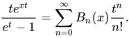
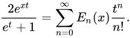
Generating functions

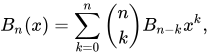
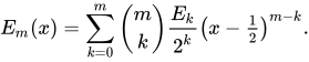
The exponential generating function for the Bernoulli polynomials is ${\frac {te^{xt}}{e^{t}-1}}=\sum _{n=0}^{\infty }B_{n}(x){\frac {t^{n}}{n!}}.$ The exponential generating function for the Euler polynomials is ${\frac {2e^{xt}}{e^{t}+1}}=\sum _{n=0}^{\infty }E_{n}(x){\frac {t^{n}}{n!}}.$

Explicit formula

$B_{n}(x)=\sum _{k=0}^{n}{n \choose k}B_{n-k}x^{k},$ $E_{m}(x)=\sum _{k=0}^{m}{m \choose k}{\frac {E_{k}}{2^{k}}}\left(x-{\tfrac {1}{2}}\right)^{m-k}.$ for $n\geq 0$ , where $B_{k}$ are the Bernoulli numbers, and $E_{k}$ are the Euler numbers. It follows that $B_{n}(0)=B_{n}$ and $E_{m}{\big (}{\tfrac {1}{2}}{\big )}={\tfrac {1}{2^{m}}}E_{m}$ .

Representation by a differential operator

The Bernoulli polynomials are also given by $\ B_{n}(x)={\frac {D}{\ e^{D}-1\ }}\ x^{n}\$ where $\ D\equiv {\frac {\mathrm {d} }{\ \mathrm {d} x\ }}\$ is differentiation with respect to x and the fraction is expanded as a formal power series. It follows that $\ \int _{a}^{x}\ B_{n}(u)\ \mathrm {d} \ u={\frac {\ B_{n+1}(x)-B_{n+1}(a)\ }{n+1}}~.$ cf. § Integrals below. By the same token, the Euler polynomials are given by $\ E_{n}(x)={\frac {2}{\ e^{D}+1\ }}\ x^{n}~.$

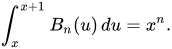
Representation by an integral operator

The Bernoulli polynomials are also the unique polynomials determined by $\int _{x}^{x+1}B_{n}(u)\,du=x^{n}.$

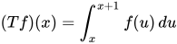
The integral transform $(Tf)(x)=\int _{x}^{x+1}f(u)\,du$ on polynomials f, simply amounts to ${\begin{aligned}(Tf)(x)={e^{D}-1 \over D}f(x)&{}=\sum _{n=0}^{\infty }{D^{n} \over (n+1)!}f(x)\\&{}=f(x)+{f'(x) \over 2}+{f''(x) \over 6}+{f'''(x) \over 24}+\cdots .\end{aligned}}$ This can be used to produce the inversion formulae below.

Integral recurrence

In, it is deduced and proved that the Bernoulli polynomials can be obtained by the following integral recurrence $B_{m}(x)=m\int _{0}^{x}B_{m-1}(t)\,dt-m\int _{0}^{1}\int _{0}^{t}B_{m-1}(s)\,dsdt.$

Another explicit formula

An explicit formula for the Bernoulli polynomials is given by $B_{n}(x)=\sum _{k=0}^{n}{\biggl [}{\frac {1}{k+1}}\sum _{\ell =0}^{k}(-1)^{\ell }{k \choose \ell }(x+\ell )^{n}{\biggr ]}.$

That is similar to the series expression for the Hurwitz zeta function in the complex plane. Indeed, there is the relationship $B_{n}(x)=-n\zeta (1-n,\,x)$ where $\zeta (s,\,q)$ is the Hurwitz zeta function. The latter generalizes the Bernoulli polynomials, allowing for non-integer values of n.

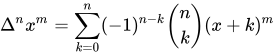
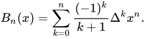
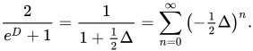
The inner sum may be understood to be the nth forward difference of $x^{m},$ that is, $\Delta ^{n}x^{m}=\sum _{k=0}^{n}(-1)^{n-k}{n \choose k}(x+k)^{m}$ where $\Delta$ is the forward difference operator. Thus, one may write $B_{n}(x)=\sum _{k=0}^{n}{\frac {(-1)^{k}}{k+1}}\Delta ^{k}x^{n}.$

This formula may be derived from an identity appearing above as follows. Since the forward difference operator Δ equals $\Delta =e^{D}-1$ where D is differentiation with respect to x, we have, from the Mercator series, ${\frac {D}{e^{D}-1}}={\frac {\log(\Delta +1)}{\Delta }}=\sum _{n=0}^{\infty }{\frac {(-\Delta )^{n}}{n+1}}.$

As long as this operates on an mth-degree polynomial such as $x^{m},$ one may let n go from 0 only up to m.

An integral representation for the Bernoulli polynomials is given by the Nörlund-Rice integral, which follows from the expression as a finite difference.

An explicit formula for the Euler polynomials is given by $E_{n}(x)=\sum _{k=0}^{n}\left[{\frac {1}{2^{k}}}\sum _{\ell =0}^{n}(-1)^{\ell }{k \choose \ell }(x+\ell )^{n}\right].$

The above follows analogously, using the fact that ${\frac {2}{e^{D}+1}}={\frac {1}{1+{\tfrac {1}{2}}\Delta }}=\sum _{n=0}^{\infty }{\bigl (}{-{\tfrac {1}{2}}}\Delta {\bigr )}^{n}.$

02Sums of pth powers

Using either the above integral representation of $x^{n}$ or the identity $B_{n}(x+1)-B_{n}(x)=nx^{n-1}$ , we have $\sum _{k=0}^{x}k^{p}=\int _{0}^{x+1}B_{p}(t)\,dt={\frac {B_{p+1}(x+1)-B_{p+1}}{p+1}}$ (assuming 0⁰ = 1).

03Explicit expressions for low degrees

The first few Bernoulli polynomials are: ${\begin{aligned}B_{0}(x)&=1,&B_{4}(x)&=x^{4}-2x^{3}+x^{2}-{\tfrac {1}{30}},\\[4mu]B_{1}(x)&=x-{\tfrac {1}{2}},&B_{5}(x)&=x^{5}-{\tfrac {5}{2}}x^{4}+{\tfrac {5}{3}}x^{3}-{\tfrac {1}{6}}x,\\[4mu]B_{2}(x)&=x^{2}-x+{\tfrac {1}{6}},&B_{6}(x)&=x^{6}-3x^{5}+{\tfrac {5}{2}}x^{4}-{\tfrac {1}{2}}x^{2}+{\tfrac {1}{42}},\\[-2mu]B_{3}(x)&=x^{3}-{\tfrac {3}{2}}x^{2}+{\tfrac {1}{2}}x{\vphantom {\Big |}},\qquad &&\ \,\,\vdots \end{aligned}}$

The first few Euler polynomials are: ${\begin{aligned}E_{0}(x)&=1,&E_{4}(x)&=x^{4}-2x^{3}+x,\\[4mu]E_{1}(x)&=x-{\tfrac {1}{2}},&E_{5}(x)&=x^{5}-{\tfrac {5}{2}}x^{4}+{\tfrac {5}{2}}x^{2}-{\tfrac {1}{2}},\\[4mu]E_{2}(x)&=x^{2}-x,&E_{6}(x)&=x^{6}-3x^{5}+5x^{3}-3x,\\[-1mu]E_{3}(x)&=x^{3}-{\tfrac {3}{2}}x^{2}+{\tfrac {1}{4}},\qquad \ \ &&\ \,\,\vdots \end{aligned}}$

04Maximum and minimum

At higher n the amount of variation in $B_{n}(x)$ between $x=0$ and $x=1$ gets large. For instance, $B_{16}(0)=B_{16}(1)={}$ $-{\tfrac {3617}{510}}\approx -7.09,$ but $B_{16}{\bigl (}{\tfrac {1}{2}}{\bigr )}={}$ ${\tfrac {118518239}{3342336}}\approx 7.09.$ Lehmer (1940) showed that the maximum value (M_n) of $B_{n}(x)$ between 0 and 1 obeys $M_{n}<{\frac {2n!}{(2\pi )^{n}}}$ unless n is 2 modulo 4, in which case $M_{n}={\frac {2\zeta (n)\,n!}{(2\pi )^{n}}}$ (where $\zeta (x)$ is the Riemann zeta function), while the minimum (m_n) obeys $m_{n}>{\frac {-2n!}{(2\pi )^{n}}}$ unless n = 0 modulo 4 , in which case $m_{n}={\frac {-2\zeta (n)\,n!}{(2\pi )^{n}}}.$

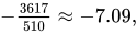
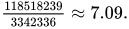
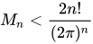
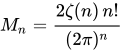
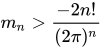
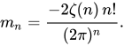
These limits are quite close to the actual maximum and minimum, and Lehmer gives more accurate limits as well.

05Differences and derivatives

The Bernoulli and Euler polynomials obey many relations from umbral calculus: ${\begin{aligned}\Delta B_{n}(x)&=B_{n}(x+1)-B_{n}(x)=nx^{n-1},\\[3mu]\Delta E_{n}(x)&=E_{n}(x+1)-E_{n}(x)=2(x^{n}-E_{n}(x)).\end{aligned}}$ (Δ is the forward difference operator). Also, $E_{n}(x+1)+E_{n}(x)=2x^{n}.$ These polynomial sequences are Appell sequences: ${\begin{aligned}B_{n}'(x)&=nB_{n-1}(x),\\[3mu]E_{n}'(x)&=nE_{n-1}(x).\end{aligned}}$

Translations

${\begin{aligned}B_{n}(x+y)&=\sum _{k=0}^{n}{n \choose k}B_{k}(x)y^{n-k}\\[3mu]E_{n}(x+y)&=\sum _{k=0}^{n}{n \choose k}E_{k}(x)y^{n-k}\end{aligned}}$ These identities are also equivalent to saying that these polynomial sequences are Appell sequences. (Hermite polynomials are another example.)

Symmetries

${\begin{aligned}B_{n}(1-x)&=\left(-1\right)^{n}B_{n}(x),&&n\geq 0,{\text{ and in particular for }}n\neq 1,~B_{n}(0)=B_{n}(1)\\[3mu]E_{n}(1-x)&=\left(-1\right)^{n}E_{n}(x)\\[1ex]\left(-1\right)^{n}B_{n}(-x)&=B_{n}(x)+nx^{n-1}\\[3mu]\left(-1\right)^{n}E_{n}(-x)&=-E_{n}(x)+2x^{n}\\[1ex]B_{n}{\bigl (}{\tfrac {1}{2}}{\bigr )}&=\left({\frac {1}{2^{n-1}}}-1\right)B_{n},&&n\geq 0{\text{ from the multiplication theorems below.}}\end{aligned}}$ Zhi-Wei Sun and Hao Pan established the following surprising symmetry relation: If r + s + t = n and x + y + z = 1, then $r[s,t;x,y]_{n}+s[t,r;y,z]_{n}+t[r,s;z,x]_{n}=0,$ where $[s,t;x,y]_{n}=\sum _{k=0}^{n}(-1)^{k}{s \choose k}{t \choose {n-k}}B_{n-k}(x)B_{k}(y).$

06Fourier series

The Fourier series of the Bernoulli polynomials is also a Dirichlet series, given by the expansion $B_{n}(x)=-{\frac {n!}{(2\pi i)^{n}}}\sum _{k\not =0}{\frac {e^{2\pi ikx}}{k^{n}}}=-2n!\sum _{k=1}^{\infty }{\frac {\cos \left(2k\pi x-{\frac {n\pi }{2}}\right)}{(2k\pi )^{n}}}.$ Note the simple large n limit to suitably scaled trigonometric functions.

This is a special case of the analogous form for the Hurwitz zeta function $B_{n}(x)=-\Gamma (n+1)\sum _{k=1}^{\infty }{\frac {\exp(2\pi ikx)+e^{i\pi n}\exp(2\pi ik(1-x))}{(2\pi ik)^{n}}}.$

This expansion is valid only for 0 ≤ x ≤ 1 when n ≥ 2 and is valid for 0 < x < 1 when n = 1.

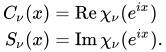
The Fourier series of the Euler polynomials may also be calculated. Defining the functions ${\begin{aligned}C_{\nu }(x)&=\sum _{k=0}^{\infty }{\frac {\cos((2k+1)\pi x)}{(2k+1)^{\nu }}}\\[3mu]S_{\nu }(x)&=\sum _{k=0}^{\infty }{\frac {\sin((2k+1)\pi x)}{(2k+1)^{\nu }}}\end{aligned}}$ for $\nu >1$ , the Euler polynomial has the Fourier series ${\begin{aligned}C_{2n}(x)&={\frac {\left(-1\right)^{n}}{4(2n-1)!}}\pi ^{2n}E_{2n-1}(x)\\[1ex]S_{2n+1}(x)&={\frac {\left(-1\right)^{n}}{4(2n)!}}\pi ^{2n+1}E_{2n}(x).\end{aligned}}$ Note that the $C_{\nu }$ and $S_{\nu }$ are odd and even, respectively: ${\begin{aligned}C_{\nu }(x)&=-C_{\nu }(1-x)\\S_{\nu }(x)&=S_{\nu }(1-x).\end{aligned}}$

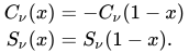
They are related to the Legendre chi function $\chi _{\nu }$ as ${\begin{aligned}C_{\nu }(x)&=\operatorname {Re} \chi _{\nu }(e^{ix})\\S_{\nu }(x)&=\operatorname {Im} \chi _{\nu }(e^{ix}).\end{aligned}}$

07Inversion

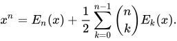
The Bernoulli and Euler polynomials may be inverted to express the monomial in terms of the polynomials.

Specifically, evidently from the above section on integral operators, it follows that $x^{n}={\frac {1}{n+1}}\sum _{k=0}^{n}{n+1 \choose k}B_{k}(x)$ and $x^{n}=E_{n}(x)+{\frac {1}{2}}\sum _{k=0}^{n-1}{n \choose k}E_{k}(x).$

08Relation to falling factorial

The Bernoulli polynomials may be expanded in terms of the falling factorial $(x)_{k}$ as $B_{n+1}(x)=B_{n+1}+\sum _{k=0}^{n}{\frac {n+1}{k+1}}\left\{{\begin{matrix}n\\k\end{matrix}}\right\}(x)_{k+1}$ where $B_{n}=B_{n}(0)$ and $\left\{{\begin{matrix}n\\k\end{matrix}}\right\}=S(n,k)$ denotes the Stirling number of the second kind. 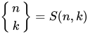The above may be inverted to express the falling factorial in terms of the Bernoulli polynomials: $(x)_{n+1}=\sum _{k=0}^{n}{\frac {n+1}{k+1}}\left[{\begin{matrix}n\\k\end{matrix}}\right]\left(B_{k+1}(x)-B_{k+1}\right)$ where $\left[{\begin{matrix}n\\k\end{matrix}}\right]=s(n,k)$ denotes the Stirling number of the first kind.

09Multiplication theorems

The multiplication theorems were given by Joseph Ludwig Raabe in 1851:

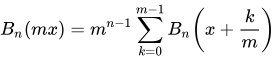
For a natural number m≥1, $B_{n}(mx)=m^{n-1}\sum _{k=0}^{m-1}B_{n}{\left(x+{\frac {k}{m}}\right)}$ ${\begin{aligned}E_{n}(mx)&=m^{n}\sum _{k=0}^{m-1}\left(-1\right)^{k}E_{n}{\left(x+{\frac {k}{m}}\right)}&{\text{ for odd }}m\\[1ex]E_{n}(mx)&={\frac {-2}{n+1}}m^{n}\sum _{k=0}^{m-1}\left(-1\right)^{k}B_{n+1}{\left(x+{\frac {k}{m}}\right)}&{\text{ for even }}m\end{aligned}}$

10Integrals

Two definite integrals relating the Bernoulli and Euler polynomials to the Bernoulli and Euler numbers are:

$\int _{0}^{1}B_{n}(t)B_{m}(t)\,dt=(-1)^{n-1}{\frac {m!\,n!}{(m+n)!}}B_{n+m}\quad {\text{for }}m,n\geq 1$
$\int _{0}^{1}E_{n}(t)E_{m}(t)\,dt=(-1)^{n}4(2^{m+n+2}-1){\frac {m!\,n!}{(m+n+2)!}}B_{n+m+2}$

Another integral formula states

$\int _{0}^{1}E_{n}\left(x+y\right)\log(\tan {\frac {\pi }{2}}x)\,dx=n!\sum _{k=1}^{\left\lfloor {\frac {n+1}{2}}\right\rfloor }{\frac {(-1)^{k-1}}{\pi ^{2k}}}\left(2-2^{-2k}\right)\zeta (2k+1){\frac {y^{n+1-2k}}{(n+1-2k)!}}$

with the special case for $y=0$

$\int _{0}^{1}E_{2n-1}\left(x\right)\log(\tan {\frac {\pi }{2}}x)\,dx={\frac {(-1)^{n-1}(2n-1)!}{\pi ^{2n}}}\left(2-2^{-2n}\right)\zeta (2n+1)$
$\int _{0}^{1}B_{2n-1}\left(x\right)\log(\tan {\frac {\pi }{2}}x)\,dx={\frac {(-1)^{n-1}}{\pi ^{2n}}}{\frac {2^{2n-2}}{(2n-1)!}}\sum _{k=1}^{n}(2^{2k+1}-1)\zeta (2k+1)\zeta (2n-2k)$
$\int _{0}^{1}E_{2n}\left(x\right)\log(\tan {\frac {\pi }{2}}x)\,dx=\int _{0}^{1}B_{2n}\left(x\right)\log(\tan {\frac {\pi }{2}}x)\,dx=0$
$\int _{0}^{1}{{{B}_{2n-1}}\left(x\right)\cot \left(\pi x\right)dx}={\frac {2\left(2n-1\right)!}{{{\left(-1\right)}^{n-1}}{{\left(2\pi \right)}^{2n-1}}}}\zeta \left(2n-1\right)$

11Periodic Bernoulli polynomials

A periodic Bernoulli polynomial P_n(x) is a Bernoulli polynomial evaluated at the fractional part of the argument x. These functions are used to provide the remainder term in the Euler-Maclaurin formula relating sums to integrals. The first polynomial is a sawtooth function.

Strictly these functions are not polynomials at all and more properly should be termed the periodic Bernoulli functions.

The following properties are of interest, valid for all $x$ :

$P_{k}(x)$ is continuous for all $k>1$
$P_{k}'(x)$ exists and is continuous for $k>2$
$P'_{k}(x)=kP_{k-1}(x)$ for $k>2$

Watch videos about Bernoulli polynomialsExplainers and documentaries on YouTube (opens in a new tab)

Sources and credits

This article is adapted from the Wikipedia article “Bernoulli polynomials”, written by its contributors and licensed under CC BY-SA 4.0. Fathomly has changed the layout, removed citation markers, navigation and maintenance notices, and adjusted punctuation. This adapted version is shared under the same license. For references, see the original article.

Images, from Wikimedia Commons:

Bernoulli polynomials.svg by The original uploader was Linas at English Wikipedia., CC BY-SA 3.0

Fathomly is not affiliated with or endorsed by the Wikimedia Foundation. Spotted a problem? Tell us.