Encyclopedia

Hadamard product (matrices)

Elementwise product of two matrices

Wikipedia contributorsAdapted for Fathomly · View authors

6 min read
Source updated August 10, 2026

In mathematics, the Hadamard product (also known as the element-wise product, entrywise product or Schur product) is a binary operation that takes in two matrices of the same dimensions and returns a matrix of the multiplied corresponding elements. This operation can be thought as a "naive matrix multiplication" and is different from the matrix product. It is attributed to, and named after, either French mathematician Jacques Hadamard or Russian mathematician Issai Schur.

The Hadamard product is associative and distributive. Unlike the matrix product, it is also commutative.

01History

Entrywise multiplication first appeared as a relevant concept in Hadamard's 1899 work on power series, where he proved the Hadamard multiplication theorem. Paul Halmos is credited for the earliest use of the term "Hadamard product" in the context of matrices, and helped popularize it. Halmos later reported that the name was suggested to him by John von Neumann and it is conjectured that it was because of the analogy with the well-known theorem of Hadamard.

02Definition

For two matrices A and B of the same dimension m × n, the Hadamard product $A\odot B$ (machine learning convention) or $A\circ B$ (matrix analysis convention) is a matrix of the same dimension as the operands, with elements given by

$(A\odot B)_{ij}=(A)_{ij}(B)_{ij}.$

For matrices of different dimensions (m × n and p × q, where m ≠ p or n ≠ q), the Hadamard product is undefined.

An example of the Hadamard product for two arbitrary 2 × 3 matrices:

${\begin{bmatrix}2&3&1\\0&8&-2\end{bmatrix}}\odot {\begin{bmatrix}3&1&4\\7&9&5\end{bmatrix}}={\begin{bmatrix}2\times 3&3\times 1&1\times 4\\0\times 7&8\times 9&-2\times 5\end{bmatrix}}={\begin{bmatrix}6&3&4\\0&72&-10\end{bmatrix}}.$

03Properties

The Hadamard product is commutative (when working with a commutative ring), associative, and distributive over addition. That is, if A, B, and C are matrices of the same size, and k is a scalar: ${\begin{aligned}A\odot B&=B\odot A,\\A\odot (B\odot C)&=(A\odot B)\odot C,\\A\odot (B+C)&=A\odot B+A\odot C,\\(kA)\odot B&=A\odot (kB)=k(A\odot B),\\A\odot 0&=0\odot A=0.\end{aligned}}$
The identity matrix under Hadamard multiplication of two m × n matrices is an m × n matrix where all elements are equal to 1. This is different from the identity matrix under regular matrix multiplication, where only the elements of the main diagonal are equal to 1. Furthermore, a matrix has an inverse under Hadamard multiplication if and only if all of the elements are invertible, or equivalently over a field, if and only if none of the elements are equal to zero.
For vectors x and y and corresponding diagonal matrices D_x and D_y with these vectors as their main diagonals, the following identity holds: $\mathbf {x} ^{*}(A\odot B)\mathbf {y} =\operatorname {tr} \left({D}_{\mathbf {x} }^{*}A{D}_{\mathbf {y} }{B}^{\mathsf {T}}\right),$ where x^* denotes the conjugate transpose of x. In particular, using vectors of ones, this shows that the sum of all elements in the Hadamard product is the trace of AB^T where superscript T denotes the matrix transpose, that is, $\operatorname {tr} \left(AB^{\mathsf {T}}\right)=\mathbf {1} ^{\mathsf {T}}\left(A\odot B\right)\mathbf {1}$ . A related result for square A and B, is that the row-sums of their Hadamard product are the diagonal elements of AB^T: $\sum _{i}(A\odot B)_{ij}=\left(B^{\mathsf {T}}A\right)_{jj}=\left(AB^{\mathsf {T}}\right)_{ii}.$ Similarly, $(\mathbf {y} \mathbf {x} ^{*})\odot A=D_{\mathbf {y} }AD_{\mathbf {x} }^{*}.$ Furthermore, a Hadamard matrix-vector product can be expressed as $(A\odot B)\mathbf {y} =\operatorname {diag} (AD_{\mathbf {y} }B^{\mathsf {T}}),$ where $\operatorname {diag} (M)$ is the vector formed from the diagonals of matrix M. Taking $\mathbf {y} =\mathbf {1}$ , this implies that $(A\odot B)\mathbf {1} =\operatorname {diag} (AB^{\mathsf {T}})$
The Hadamard product is a principal submatrix of the Kronecker product.
The Hadamard product satisfies the rank inequality $\operatorname {rank} (A\odot B)\leq \operatorname {rank} (A)\operatorname {rank} (B).$
If A and B are positive-definite matrices, then the following inequality involving the Hadamard product holds: $\prod _{i=k}^{n}\lambda _{i}(A\odot B)\geq \prod _{i=k}^{n}\lambda _{i}(AB),\quad k=1,\ldots ,n,$ where λ_i(A) is the ith largest eigenvalue of A.
If D and E are diagonal matrices, then ${\begin{aligned}D(A\odot B)E&=(DAE)\odot B=(DA)\odot (BE)\\&=(AE)\odot (DB)=A\odot (DBE).\end{aligned}}$
The Hadamard product of two vectors $\mathbf {a}$ and $\mathbf {b}$ is the same as matrix multiplication of the corresponding diagonal matrix of one vector by the other vector: $\mathbf {a} \odot \mathbf {b} =D_{\mathbf {a} }\mathbf {b} =D_{\mathbf {b} }\mathbf {a} .$
The $\operatorname {diag}$ operator transforming a vector to a diagonal matrix may be expressed using the Hadamard product as $\operatorname {diag} (\mathbf {a} )=(\mathbf {a} \mathbf {1} ^{T})\odot I,$ where $\mathbf {1}$ is a constant vector with elements $1$ , and $I$ is the identity matrix.

04The mixed-product property

The Hadamard product obeys certain relationships with other matrix product operators.

If $\otimes$ is the Kronecker product, assuming $A$ has the same dimensions as $C$ and $B$ as $D$ , then $(A\otimes B)\odot (C\otimes D)=(A\odot C)\otimes (B\odot D).$

If $\bullet$ is the face-splitting product, then $(A\bullet B)\odot (C\bullet D)=(A\odot C)\bullet (B\odot D).$

If $\ast$ is the column-wise Khatri-Rao product, then $(A\bullet B)(C\ast D)=(AC)\odot (BD).$

05Schur product theorem

The Hadamard product of two positive-semidefinite matrices is positive-semidefinite. This is known as the Schur product theorem, after Russian mathematician Issai Schur. For two positive-semidefinite matrices A and B, it is also known that the determinant of their Hadamard product is greater than or equal to the product of their respective determinants: $\det({A}\odot {B})\geq \det({A})\det({B}).$

06Analogous operations

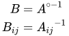
Other Hadamard operations are also seen in the mathematical literature, namely the Hadamard root and Hadamard power (which are in effect the same thing because of fractional indices), defined for a matrix such that:

For ${\begin{aligned}{B}&={A}^{\circ 2}\\B_{ij}&={A_{ij}}^{2}\end{aligned}}$

and for ${\begin{aligned}{B}&={A}^{\circ {\frac {1}{2}}}\\B_{ij}&={A_{ij}}^{\frac {1}{2}}\end{aligned}}$

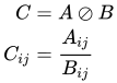
The Hadamard inverse reads: ${\begin{aligned}{B}&={A}^{\circ -1}\\B_{ij}&={A_{ij}}^{-1}\end{aligned}}$

A Hadamard division is defined as:

${\begin{aligned}{C}&={A}\oslash {B}\\C_{ij}&={\frac {A_{ij}}{B_{ij}}}\end{aligned}}$

07In programming languages

Most scientific or numerical programming languages include the Hadamard product, under various names.

In MATLAB, the Hadamard product is expressed as "dot multiply": a .* b, or the function call: times(a, b). It also has analogous dot operators which include, for example, the operators a .^ b and a ./ b. Because of this mechanism, it is possible to reserve * and ^ for matrix multiplication and matrix exponentials, respectively.

The programming language Julia has similar syntax as MATLAB, where Hadamard multiplication is called broadcast multiplication and also denoted with a .* b, and other operators are analogously defined element-wise, for example Hadamard powers use a .^ b. But unlike MATLAB, in Julia this "dot" syntax is generalized with a generic broadcasting operator . which can apply any function element-wise. This includes both binary operators (such as the aforementioned multiplication and exponentiation, as well as any other binary operator such as the Kronecker product), and also unary operators such as ! and √. Thus, any function in prefix notation f can be applied as f.(x).

Python does not have built-in array support, leading to inconsistent/conflicting notations. The NumPy numerical library interprets a*b or a.multiply(b) as the Hadamard product, and uses a@b or a.matmul(b) for the matrix product. With the SymPy symbolic library, multiplication of array objects as either a*b or a@b will produce the matrix product. The Hadamard product can be obtained with the method call a.multiply_elementwise(b). Some Python packages include support for Hadamard powers using methods like np.power(a, b), or the Pandas method a.pow(b).

In C++, the Eigen library provides a cwiseProduct member function for the Matrix class (a.cwiseProduct(b)), while the Armadillo library uses the operator % to make compact expressions (a % b; a * b is a matrix product).

In GAUSS, and HP Prime, the operation is known as array multiplication.

In Fortran, R, APL, J, and Wolfram Language (Mathematica), the multiplication operator * or × apply the Hadamard product, whereas the matrix product is written using matmul, %*%, +.×, +/ .* and ., respectively.

In the Maple programming language, the multiplication operator * is not defined for Matrices and Vectors. The matrix product is written using ., while the Hadamard product may be obtained using *~. (The ~ is a 'broadcast operator' similar to . in Julia.)

The R package matrixcalc introduces the function hadamard.prod() for Hadamard Product of numeric matrices or vectors.

The computer algebra system Maxima uses . for matrix multiplication and * for the Hadamard Product.

08Applications

The Hadamard product appears in lossy compression algorithms such as JPEG. The decoding step involves an entry-for-entry product, in other words the Hadamard product.

In image processing, the Hadamard operator can be used for enhancing, suppressing or masking image regions. One matrix represents the original image, the other acts as weight or masking matrix.

It is used in the machine learning literature, for example, to describe the architecture of recurrent neural networks as GRUs or LSTMs.

It is also used to study the statistical properties of random vectors and matrices.

09The penetrating face product

According to the definition of V. Slyusar the penetrating face product of the p×g matrix ${A}$ and n-dimensional matrix ${B}$ (n > 1) with p×g blocks ( ${B}=[B_{n}]$ ) is a matrix of size ${B}$ of the form: ${A}[\circ ]{B}=\left[{\begin{array}{c | c | c | c }{A}\circ {B}_{1}&{A}\circ {B}_{2}&\cdots &{A}\circ {B}_{n}\end{array}}\right].$

Example

If ${A}={\begin{bmatrix}1&2&3\\4&5&6\\7&8&9\end{bmatrix}},\quad {B}=\left[{\begin{array}{c | c | c }{B}_{1}&{B}_{2}&{B}_{3}\end{array}}\right]=\left[{\begin{array}{c c c | c c c | c c c }1&4&7&2&8&14&3&12&21\\8&20&5&10&25&40&12&30&6\\2&8&3&2&4&2&7&3&9\end{array}}\right]$

then

${A}[\circ ]{B}=\left[{\begin{array}{c c c | c c c | c c c }1&8&21&2&16&42&3&24&63\\32&100&30&40&125&240&48&150&36\\14&64&27&14&32&18&49&24&81\end{array}}\right].$

Main properties

${A}[\circ ]{B}={B}[\circ ]{A};$

${M}\bullet {M}={M}[\circ ]\left({M}\otimes \mathbf {1} ^{\textsf {T}}\right),$

where $\bullet$ denotes the face-splitting product of matrices,

$\mathbf {c} \bullet {M}=\mathbf {c} [\circ ]{M},$ where $\mathbf {c}$ is a vector.

Applications

The penetrating face product is used in the tensor-matrix theory of digital antenna arrays. This operation can also be used in artificial neural network models, specifically convolutional layers.

Watch videos about Hadamard product (matrices)Explainers and documentaries on YouTube (opens in a new tab)

Sources and credits

This article is adapted from the Wikipedia article “Hadamard product (matrices)”, written by its contributors and licensed under CC BY-SA 4.0. Fathomly has changed the layout, removed citation markers, navigation and maintenance notices, and adjusted punctuation. This adapted version is shared under the same license. For references, see the original article.

Images, from Wikimedia Commons:

Hadamard product qtl1.svg by Quartl, CC BY-SA 3.0
Penetrating face product.jpg by Swadim, CC BY-SA 4.0

Fathomly is not affiliated with or endorsed by the Wikimedia Foundation. Spotted a problem? Tell us.