Encyclopedia

Einstein coefficients

Quantities describing probability of absorption or emission of light

Wikipedia contributorsAdapted for Fathomly · View authors

8 min read
Source updated July 27, 2026

Image credit is listed at the end of this article.

In atomic, molecular, and optical physics, the Einstein coefficients are quantities describing the probability of absorption or emission of a photon by an atom or molecule. The Einstein A coefficients are related to the rate of spontaneous emission of light, and the Einstein B coefficients are related to the absorption and stimulated emission of light. Throughout this article, "light" refers to any electromagnetic radiation, not necessarily in the visible spectrum.

These coefficients are named after Albert Einstein, who proposed them in 1916.

01History

In the 19th century there were many measurements of the amount of light absorbed by a various gases as the incoming light frequency was varied, called absorption spectra, and measurements of the light emitted from gases energized by, for example flames, called emission spectra. To the end of that century it was believed that these spectra were caused by vibrations of atoms. In 1907 Arthur William Conway proposed instead that a change in the electron state of a single electron creates a single line. Then the many characteristic lines in the spectra resulted from many atoms with electrons in a variety of different states.

Better models for the atom appeared after Ernest Rutherford showed that they contained a concentrated atomic nucleus surrounded by electrons. John William Nicholson proposed in 1911 that the characteristic lines represented transitions of electrons limited to discrete changes in angular momentum. Then in 1913, Niels Bohr developed a complete model for quantized transitions between electron energy levels that substantially reproduced the atomic spectral line observations.

In Bohr's model a photon with an energy equal to the difference E₂ − E₁ between two energy levels is released or absorbed by an atom. The frequency ν at which the spectral line occurs is related to the photon energy by Bohr's frequency condition E₂ − E₁ = hν where h denotes the Planck constant. Bohr's theory related the states of atoms to the energy of the characteristic lines, but it said nothing about why some lines are strong and others weak.

Albert Einstein introduced the coefficients in 1916 and 1917 in a series of papers outlining his quantum theory of radiation interacting with matter. Einstein adopted one quantum assumption from Bohr's model of the atoms, that they exist in stationary states. Each state has an energy. Einstein treats the interaction between these atoms and a radiation field using Max Planck's classical oscillator, in effect replacing the non-specific oscillators of Planck's law with Bohr atoms. The relative phase of an oscillator and electromagnetic field determines the direction energy flows during the interaction. The probability of interaction is proportional to the spectral flux density of the electromagnetic field, $\rho (\nu ,T).$ Assuming just two energy levels, $E_{b}>E_{a}$ , absorption corresponds to $a\rightarrow b$ with proportionality constant, $B_{ab}$ , and emission corresponds to $b\rightarrow a$ with proportionality constant, $B_{ba}$ . This type of emission came to be called stimulated emission. Einstein adds a third constant, $A_{ba}$ , independent of the flux density, corresponding to spontaneous emission in the absence of the field.

Paul Dirac derived the coefficients in a 1927 paper titled "The Quantum Theory of the Emission and Absorption of Radiation".

02Emission and absorption coefficients

Spontaneous emission

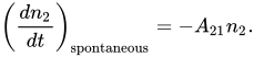
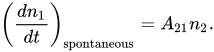
Spontaneous emission is the process by which an electron "spontaneously" (i.e., without any outside influence) decays from a higher energy level to a lower one. The process is described by the Einstein coefficient A₂₁ (s⁻¹), which gives the probability per unit time that an electron in state 2 with energy $E_{2}$ will decay spontaneously to state 1 with energy $E_{1}$ , emitting a photon with an energy E₂ − E₁ = hν. Due to the energy-time uncertainty principle, the transition actually produces photons within a narrow range of frequencies called the spectral linewidth. If $n_{i}$ is the volumetric number density of atoms in state i, then the change in the number density of atoms in state 2 per unit time due to spontaneous emission will be $\left({\frac {dn_{2}}{dt}}\right)_{\text{spontaneous}}=-A_{21}n_{2}.$

The same process results in an increase in the population of state 1: $\left({\frac {dn_{1}}{dt}}\right)_{\text{spontaneous}}=A_{21}n_{2}.$

Stimulated emission

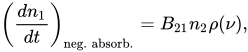
Stimulated emission (also known as induced emission) is the process by which an electron is induced to jump from a higher energy level to a lower one by the presence of electromagnetic radiation at (or near) the frequency of the transition. From the thermodynamic viewpoint, this process must be regarded as negative absorption. The process is described by the Einstein coefficient $B_{21}$ (m³ J⁻¹ s⁻²), which gives the probability per unit time per unit energy density of the radiation field per unit frequency that an electron in state 2 with energy $E_{2}$ will decay to state 1 with energy $E_{1}$ , emitting a photon with an energy E₂ − E₁ = hν. The change in the number density of atoms in state 1 per unit time due to induced emission will be $\left({\frac {dn_{1}}{dt}}\right)_{\text{neg. absorb.}}=B_{21}n_{2}\rho (\nu ),$ where $\rho (\nu )$ denotes the spectral energy density of the isotropic radiation field at the frequency of the transition (see Planck's law).

Stimulated emission is one of the fundamental processes that led to the development of the laser. Laser radiation is, however, very far from the present case of isotropic radiation.

Absorption

Absorption is the process by which a photon is absorbed by the atom, causing an electron to jump from a lower energy level to a higher one. The process is described by the Einstein coefficient $B_{12}$ (m³ J⁻¹ s⁻²), which gives the probability per unit time per unit energy density of the radiation field per unit frequency that an electron in state 1 with energy $E_{1}$ will absorb a photon with an energy E₂ − E₁ = hν and jump to state 2 with energy $E_{2}$ . The change in the number density of atoms in state 1 per unit time due to absorption will be $\left({\frac {dn_{1}}{dt}}\right)_{\text{pos. absorb.}}=-B_{12}n_{1}\rho (\nu ).$

Units

Different authors use different units for frequency-dependent quantities. In particular, the spectral energy density can be expressed per unit of frequency, angular frequency, energy (e.g., electronvolt), or wavelength. Consequently, the $B_{12}$ and $B_{21}$ coefficients will have different units. This is sometimes indicated (e.g., $B_{21}^{\omega }$ ), but more often silently omitted. The $A_{21}$ coefficient remains in the units of 1/time.

Schematic diagram of atomic stimulated emission

03Detailed balance

The Einstein coefficients are fixed probabilities per time associated with each atom, and do not depend on the state of the gas of which the atoms are a part. Therefore, any relationship that we can derive between the coefficients at, say, thermodynamic equilibrium will be valid universally.

At thermodynamic equilibrium, we will have a simple balancing, in which the net change in the number of any excited atoms is zero, being balanced by loss and gain due to all processes. With respect to bound-bound transitions, we will have detailed balancing as well, which states that the net exchange between any two levels will be balanced. This is because the probabilities of transition cannot be affected by the presence or absence of other excited atoms. Detailed balance (valid only at equilibrium) requires that the change in time of the number of atoms in level 1 due to the above three processes be zero: $0=A_{21}n_{2}+B_{21}n_{2}\rho (\nu )-B_{12}n_{1}\rho (\nu ).$

Along with detailed balancing, at temperature T we may use our knowledge of the equilibrium energy distribution of the atoms, as stated in the Maxwell-Boltzmann distribution, and the equilibrium distribution of the photons, as stated in Planck's law of black body radiation to derive universal relationships between the Einstein coefficients.

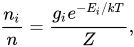
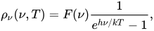
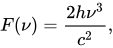
From Boltzmann distribution we have for the number of excited atomic species i: ${\frac {n_{i}}{n}}={\frac {g_{i}e^{-E_{i}/kT}}{Z}},$ where n is the total number density of the atomic species, excited and unexcited, k is the Boltzmann constant, T is the temperature, $g_{i}$ is the degeneracy (also called the multiplicity) of state i, and Z is the partition function. From Planck's law of black-body radiation at temperature T we have for the spectral radiance (radiance is energy per unit time per unit solid angle per unit projected area, when integrated over an appropriate spectral interval) at frequency ν $\rho _{\nu }(\nu ,T)=F(\nu ){\frac {1}{e^{h\nu /kT}-1}},$ where $F(\nu )={\frac {2h\nu ^{3}}{c^{2}}},$ where $c$ is the speed of light and $h$ is the Planck constant.

Substituting these expressions into the equation of detailed balancing and remembering that E₂ − E₁ = hν yields $A_{21}g_{2}e^{-h\nu /kT}+B_{21}g_{2}e^{-h\nu /kT}{\frac {F(\nu )}{e^{h\nu /kT}-1}}=B_{12}g_{1}{\frac {F(\nu )}{e^{h\nu /kT}-1}},$ or $A_{21}g_{2}(1-e^{-h\nu /kT})+B_{21}g_{2}F(\nu )e^{-h\nu /kT}=B_{12}g_{1}F(\nu ).$

The above equation must hold at any temperature, so from $T\to \infty$ one gets $B_{21}g_{2}=B_{12}g_{1},$ and from $T\to 0$ $A_{21}g_{2}=B_{21}g_{2}F(\nu ).$

Therefore, the three Einstein coefficients are interrelated by ${\frac {A_{21}}{B_{21}}}=F(\nu )$ and ${\frac {B_{21}}{B_{12}}}={\frac {g_{1}}{g_{2}}}.$

When this relation is inserted into the original equation, one can also find a relation between $A_{21}$ and $B_{12}$ , involving Planck's law.

04Oscillator strengths

The oscillator strength $f_{12}$ is defined by the following relation to the cross section $\sigma$ for absorption: $\sigma ={\frac {e^{2}}{4\varepsilon _{0}m_{e}c}}\,f_{12}\,\phi _{\nu }={\frac {\pi e^{2}}{2\varepsilon _{0}m_{e}c}}\,f_{12}\,\phi _{\omega },$

where $e$ is the electron charge, $m_{e}$ is the electron mass, and $\phi _{\nu }$ and $\phi _{\omega }$ are normalized distribution functions in frequency and angular frequency respectively. This allows all three Einstein coefficients to be expressed in terms of the single oscillator strength associated with the particular atomic spectral line: ${\begin{aligned}B_{12}&={\frac {e^{2}}{4\varepsilon _{0}m_{e}h\nu }}f_{12},\\[1ex]B_{21}&={\frac {e^{2}}{4\varepsilon _{0}m_{e}h\nu }}{\frac {g_{1}}{g_{2}}}f_{12},\\[1ex]A_{21}&={\frac {2\pi \nu ^{2}e^{2}}{\varepsilon _{0}m_{e}c^{3}}}{\frac {g_{1}}{g_{2}}}f_{12}.\end{aligned}}$

05Dipole approximation

The value of A and B coefficients can be calculated using quantum mechanics where dipole approximations in time dependent perturbation theory is used. While the calculation of B coefficient can be done easily, that of A coefficient requires using results of second quantization. This is because the theory developed by dipole approximation and time dependent perturbation theory gives a semiclassical description of electronic transition which goes to zero as perturbing fields go to zero. The A coefficient which governs spontaneous emission should not go to zero as perturbing fields go to zero. 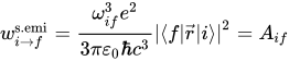The result for transition rates of different electronic levels as a result of spontaneous emission is given as (in SI units): $w_{i\to f}^{\text{s.emi}}={\frac {\omega _{if}^{3}e^{2}}{3\pi \varepsilon _{0}\hbar c^{3}}}\left|\langle f|{\vec {r}}|i\rangle \right|^{2}=A_{if}$

For B coefficient, straightforward application of dipole approximation in time dependent perturbation theory yields (in SI units): $w_{i\rightarrow f}^{\text{abs}}={\frac {u(\omega _{fi})\pi e^{2}}{3\varepsilon _{0}\hbar ^{2}}}\left|\langle f|{\vec {r}}|i\rangle \right|^{2}=B_{if}^{\text{abs}}u(\omega _{fi})$ $w_{i\to f}^{\text{emi}}={\frac {u(\omega _{if})\pi e^{2}}{3\varepsilon _{0}\hbar ^{2}}}\left|\langle f|{\vec {r}}|i\rangle \right|^{2}=B_{if}^{emi}u(\omega _{if})$

Note that the rate of transition formula depends on dipole moment operator. For higher order approximations, it involves quadrupole moment and other similar terms.

Here, the B coefficients are chosen to correspond to $\omega$ energy distribution function. Often these different definitions of B coefficients are distinguished by superscript, for example, ${\textstyle B_{21}^{f}={\frac {B_{21}^{\omega }}{2\pi }}$ where ${\textstyle B_{21}^{f}$ term corresponds to frequency distribution and ${\textstyle B_{21}^{\omega }$ term corresponds to $\omega$ distribution. The formulas for B coefficients varies inversely to that of the energy distribution chosen, so that the transition rate is same regardless of convention.

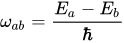
Hence, AB coefficients are calculated using dipole approximation as: ${\begin{aligned}A_{ab}&={\frac {\omega _{ab}^{3}e^{2}}{3\pi \varepsilon _{0}\hbar c^{3}}}\left|\langle a|{\vec {r}}|b\rangle \right|^{2}\\[1ex]B_{ab}&={\frac {\pi e^{2}}{3\varepsilon _{0}\hbar ^{2}}}\left|\langle a|{\vec {r}}|b\rangle \right|^{2}\end{aligned}}$ where $\omega _{ab}={\frac {E_{a}-E_{b}}{\hbar }}$ and B coefficients correspond to $\omega$ energy distribution function.

Hence the following ratios are also derived: ${\frac {B_{12}}{B_{21}}}=1$ and ${\frac {A_{if}}{B}}={\frac {\omega _{if}^{3}\hbar }{\pi ^{2}c^{3}}}$

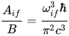
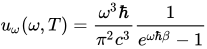
Derivation of Planck's law

It follows from theory that: ${\frac {dN_{b}}{dt}}=-A_{ba}N_{b}-N_{b}u(\omega _{ba})B_{ba}+N_{a}u(\omega _{ba})B_{ab}=-N_{b}w_{b\to a}^{\text{s.emi}}-N_{b}w_{b\to a}^{\text{emi}}+N_{a}w_{a\to b}^{\text{abs}}$ where $N_{a}$ and $N_{b}$ are number of occupied energy levels of $E_{a}$ and $E_{b}$ respectively, where $E_{b}>E_{a}$ . Note that from time dependent perturbation theory application, the fact that only radiation whose $\omega$ is close to value of $\omega _{ba}$ can produce respective stimulated emission or absorption, is used.

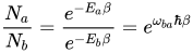
Where Maxwell distribution involving $N_{a}$ and $N_{b}$ ensures ${\frac {N_{a}}{N_{b}}}={\frac {e^{-E_{a}\beta }}{e^{-E_{b}\beta }}}=e^{\omega _{ba}\hbar \beta }$

Solving for $u$ for equilibrium condition ${\frac {dN_{b}}{dt}}=0$ using the above equations and ratios while generalizing $\omega _{ba}$ to $\omega$ , we get: $u_{\omega }(\omega ,T)={\frac {\omega ^{3}\hbar }{\pi ^{2}c^{3}}}{\frac {1}{e^{\omega \hbar \beta }-1}}$ which is the angular frequency energy distribution from Planck's law.

Watch videos about Einstein coefficientsExplainers and documentaries on YouTube (opens in a new tab)

Sources and credits

This article is adapted from the Wikipedia article “Einstein coefficients”, written by its contributors and licensed under CC BY-SA 4.0. Fathomly has changed the layout, removed citation markers, navigation and maintenance notices, and adjusted punctuation. This adapted version is shared under the same license. For references, see the original article.

Images, from Wikimedia Commons:

Spectral lines en.PNG by User:Jhausauer, Public domain
AtomicLineSpEm.svg by Cwbm (commons), GPLv3
AtomicLineInEm.svg by Krishnavedala, CC0
AtomicLineAb.svg by Krishnavedala, CC0

Fathomly is not affiliated with or endorsed by the Wikimedia Foundation. Spotted a problem? Tell us.