Encyclopedia

Darwin-Fowler method

Method for deriving the distribution functions with mean probability

Wikipedia contributorsAdapted for Fathomly · View authors

4 min read
Source updated March 21, 2026

In statistical mechanics, the Darwin-Fowler method is used for deriving distribution functions with mean probability. It was developed by Charles Galton Darwin and Ralph H. Fowler in 1922-1923.

Distribution functions are used in statistical physics to estimate the mean number of particles occupying an energy level (hence also called occupation numbers). These distributions are mostly derived as those numbers for which the system under consideration is in its state of maximum probability. But one really requires average numbers. These average numbers can be obtained by the Darwin-Fowler method. Of course, for systems in the thermodynamic limit (large number of particles), as in statistical mechanics, the results are the same as with maximization.

01Darwin-Fowler method

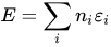
In most texts on statistical mechanics the statistical distribution functions $f$ in Maxwell-Boltzmann statistics, Bose-Einstein statistics, Fermi-Dirac statistics) are derived by determining those for which the system is in its state of maximum probability. But one really requires those with average or mean probability, although, of course, the results are usually the same for systems with a huge number of elements, as is the case in statistical mechanics. The method for deriving the distribution functions with mean probability has been developed by C. G. Darwin and Fowler and is therefore known as the Darwin-Fowler method. This method is the most reliable general procedure for deriving statistical distribution functions. Since the method employs a selector variable (a factor introduced for each element to permit a counting procedure) the method is also known as the Darwin-Fowler method of selector variables. Note that a distribution function is not the same as the probability, cf. Maxwell-Boltzmann distribution, Bose-Einstein distribution, Fermi-Dirac distribution. Also note that the distribution function $f_{i}$ which is a measure of the fraction of those states which are actually occupied by elements, is given by $f_{i}=n_{i}/g_{i}$ or $n_{i}=f_{i}g_{i}$ , where $g_{i}$ is the degeneracy of energy level $i$ of energy $\varepsilon _{i}$ and $n_{i}$ is the number of elements occupying this level (e.g. in Fermi-Dirac statistics 0 or 1). Total energy $E$ and total number of elements $N$ are then given by $E=\sum _{i}n_{i}\varepsilon _{i}$ and $N=\sum n_{i}$ .

The Darwin-Fowler method has been treated in the texts of E. Schrödinger, Fowler and Fowler and E. A. Guggenheim, of K. Huang, and of H. J. W. Müller-Kirsten. The method is also discussed and used for the derivation of Bose-Einstein condensation in the book of R. B. Dingle.

02Classical statistics

For $N=\sum _{i}n_{i}$ independent elements with $n_{i}$ on level with energy $\varepsilon _{i}$ and $E=\sum _{i}n_{i}\varepsilon _{i}$ for a canonical system in a heat bath with temperature $T$ we set

$Z=\sum _{\text{arrangements}}e^{-E/kT}=\sum _{\text{arrangements}}\prod _{i}z_{i}^{n_{i}},\;\;\;z_{i}=e^{-\varepsilon _{i}/kT}.$

The average over all arrangements is the mean occupation number

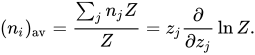
$(n_{i})_{\text{av}}={\frac {\sum _{j}n_{j}Z}{Z}}=z_{j}{\frac {\partial }{\partial z_{j}}}\ln Z.$

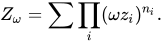
Insert a selector variable $\omega$ by setting

$Z_{\omega }=\sum \prod _{i}(\omega z_{i})^{n_{i}}.$

In classical statistics the $N$ elements are (a) distinguishable and can be arranged with packets of $n_{i}$ elements on level $\varepsilon _{i}$ whose number is

${\frac {N!}{\prod _{i}n_{i}!}},$

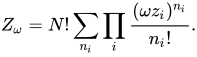
so that in this case

$Z_{\omega }=N!\sum _{n_{i}}\prod _{i}{\frac {(\omega z_{i})^{n_{i}}}{n_{i}!}}.$

Allowing for (b) the degeneracy $g_{i}$ of level $\varepsilon _{i}$ this expression becomes

$Z_{\omega }=N!\prod _{i=1}^{\infty }\left(\sum _{n_{i}=0,1,2,\ldots }{\frac {(\omega z_{i})^{n_{i}}}{n_{i}!}}\right)^{g_{i}}=N!e^{\omega \sum _{i}g_{i}z_{i}}.$

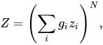
The selector variable $\omega$ allows one to pick out the coefficient of $\omega ^{N}$ which is $Z$ . Thus

$Z=\left(\sum _{i}g_{i}z_{i}\right)^{N},$

and hence

$(n_{j})_{\text{av}}=z_{j}{\frac {\partial }{\partial z_{j}}}\ln Z=N{\frac {g_{j}e^{-\varepsilon _{j}/kT}}{\sum _{i}g_{i}e^{-\varepsilon _{i}/kT}}}.$

This result which agrees with the most probable value obtained by maximization does not involve a single approximation and is therefore exact, and thus demonstrates the power of this Darwin-Fowler method.

03Quantum statistics

We have as above

$Z_{\omega }=\sum \prod (\omega z_{i})^{n_{i}},\;\;z_{i}=e^{-\varepsilon _{i}/kT},$

where $n_{i}$ is the number of elements in energy level $\varepsilon _{i}$ . Since in quantum statistics elements are indistinguishable no preliminary calculation of the number of ways of dividing elements into packets $n_{1},n_{2},n_{3},...$ is required. Therefore, the sum $\sum$ refers only to the sum over possible values of $n_{i}$ .

In the case of Fermi-Dirac statistics we have

$n_{i}=0$ or $n_{i}=1$

per state. There are $g_{i}$ states for energy level $\varepsilon _{i}$ . Hence we have

$Z_{\omega }=(1+\omega z_{1})^{g_{1}}(1+\omega z_{2})^{g_{2}}\cdots =\prod (1+\omega z_{i})^{g_{i}}.$

In the case of Bose-Einstein statistics we have

$n_{i}=0,1,2,3,\ldots \infty .$

By the same procedure as before we obtain in the present case

$Z_{\omega }=(1+\omega z_{1}+(\omega z_{1})^{2}+(\omega z_{1})^{3}+\cdots )^{g_{1}}(1+\omega z_{2}+(\omega z_{2})^{2}+\cdots )^{g_{2}}\cdots .$

But

$1+\omega z_{1}+(\omega z_{1})^{2}+\cdots ={\frac {1}{(1-\omega z_{1})}}.$

Therefore

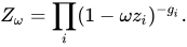
$Z_{\omega }=\prod _{i}(1-\omega z_{i})^{-g_{i}}.$

Summarizing both cases and recalling the definition of $Z$ , we have that $Z$ is the coefficient of $\omega ^{N}$ in

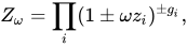
$Z_{\omega }=\prod _{i}(1\pm \omega z_{i})^{\pm g_{i}},$

where the upper signs apply to Fermi-Dirac statistics, and the lower signs to Bose-Einstein statistics.

Next we have to evaluate the coefficient of $\omega ^{N}$ in $Z_{\omega }.$ In the case of a function $\phi (\omega )$ which can be expanded as

$\phi (\omega )=a_{0}+a_{1}\omega +a_{2}\omega ^{2}+\cdots ,$

the coefficient of $\omega ^{N}$ is, with the help of the residue theorem of Cauchy,

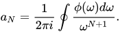
$a_{N}={\frac {1}{2\pi i}}\oint {\frac {\phi (\omega )d\omega }{\omega ^{N+1}}}.$

We note that similarly the coefficient $Z$ in the above can be obtained as

$Z={\frac {1}{2\pi i}}\oint {\frac {Z_{\omega }}{\omega ^{N+1}}}d\omega \equiv {\frac {1}{2\pi i}}\int e^{f(\omega )}d\omega ,$

where

$f(\omega )=\pm \sum _{i}g_{i}\ln(1\pm \omega z_{i})-(N+1)\ln \omega .$

Differentiating one obtains

$f'(\omega )={\frac {1}{\omega }}\left[\sum _{i}{\frac {g_{i}}{(\omega z_{i})^{-1}\pm 1}}-(N+1)\right],$

and

$f''(\omega )={\frac {N+1}{\omega ^{2}}}\mp {\frac {1}{\omega ^{2}}}\sum _{i}{\frac {g_{i}}{[(\omega z_{i})^{-1}\pm 1]^{2}}}.$

One now evaluates the first and second derivatives of $f(\omega )$ at the stationary point $\omega _{0}$ at which $f'(\omega _{0})=0.$ . This method of evaluation of $Z$ around the saddle point $\omega _{0}$ is known as the method of steepest descent. One then obtains

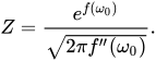
$Z={\frac {e^{f(\omega _{0})}}{\sqrt {2\pi f''(\omega _{0})}}}.$

We have $f'(\omega _{0})=0$ and hence

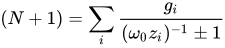
$(N+1)=\sum _{i}{\frac {g_{i}}{(\omega _{0}z_{i})^{-1}\pm 1}}$

(the +1 being negligible since $N$ is large). We shall see in a moment that this last relation is simply the formula

$N=\sum _{i}n_{i}.$

We obtain the mean occupation number $(n_{i})_{av}$ by evaluating

$(n_{j})_{av}=z_{j}{\frac {d}{dz_{j}}}\ln Z={\frac {g_{j}}{(\omega _{0}z_{j})^{-1}\pm 1}}={\frac {g_{j}}{e^{(\varepsilon _{j}-\mu )/kT}\pm 1}},\quad e^{\mu /kT}=\omega _{0}.$

This expression gives the mean number of elements of the total of $N$ in the volume $V$ which occupy at temperature $T$ the 1-particle level $\varepsilon _{j}$ with degeneracy $g_{j}$ (see e.g. a priori probability). For the relation to be reliable one should check that higher order contributions are initially decreasing in magnitude so that the expansion around the saddle point does indeed yield an asymptotic expansion.

Watch videos about Darwin-Fowler methodExplainers and documentaries on YouTube (opens in a new tab)

Sources and credits

This article is adapted from the Wikipedia article “Darwin-Fowler method”, written by its contributors and licensed under CC BY-SA 4.0. Fathomly has changed the layout, removed citation markers, navigation and maintenance notices, and adjusted punctuation. This adapted version is shared under the same license. For references, see the original article.

Fathomly is not affiliated with or endorsed by the Wikimedia Foundation. Spotted a problem? Tell us.