Encyclopedia

Conditional independence

Probability theory concept

Wikipedia contributorsAdapted for Fathomly · View authors

7 min read
Source updated May 25, 2026

In probability theory, conditional independence describes situations in which an observation is irrelevant or redundant when evaluating the certainty of a hypothesis. It is the opposite of conditional dependence. Conditional independence is usually formulated in terms of conditional probability, as a special case where the probability of the hypothesis given the uninformative observation is equal to the probability without. If $A$ is the hypothesis, and $B$ and $C$ are observations, conditional independence can be stated as an equality:

$P(A\mid B,C)=P(A\mid C)$

where $P(A\mid B,C)$ is the probability of $A$ given both $B$ and $C$ . Since the probability of $A$ given $C$ is the same as the probability of $A$ given both $B$ and $C$ , this equality expresses that $B$ contributes nothing to the certainty of $A$ . In this case, $A$ and $B$ are said to be conditionally independent given $C$ , written symbolically as: $(A\perp \!\!\!\perp B\mid C)$ .

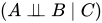
The concept of conditional independence is essential to graph-based theories of statistical inference, as it establishes a mathematical relation between a collection of conditional statements and a graphoid.

01Conditional independence of events

Let $A$ , $B$ , and $C$ be events. $A$ and $B$ are said to be conditionally independent given $C$ if and only if $P(C)>0$ and $P(A\mid B,C)=P(A\mid C)$ . This property is symmetric (more on this below) and often written as $(A\perp \!\!\!\perp B\mid C)$ , which should be read as $((A\perp \!\!\!\perp B)\vert C)$ .

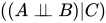
Equivalently, conditional independence may be stated as $P(A,B|C)=P(A|C)P(B|C)$ where $P(A,B|C)$ is the joint probability of $A$ and $B$ given $C$ . This alternate formulation states that $A$ and $B$ are independent events, given $C$ .

It demonstrates that 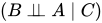$(A\perp \!\!\!\perp B\mid C)$ is equivalent to $(B\perp \!\!\!\perp A\mid C)$ .

Proof of the equivalent definition

${\begin{aligned}P(A,B\mid C)=P(A\mid C)P(B\mid C)&\iff {\frac {P(A,B,C)}{P(C)}}=\left({\frac {P(A,C)}{P(C)}}\right)\left({\frac {P(B,C)}{P(C)}}\right)&{\text{definition of conditional probability}}\\&\iff P(A,B,C)={\frac {P(A,C)P(B,C)}{P(C)}}&{\text{multiply both sides by P(C)}}\\&\iff {\frac {P(A,B,C)}{P(B,C)}}={\frac {P(A,C)}{P(C)}}&{\text{divide both sides by P(B, C)}}\\&\iff P(A\mid B,C)=P(A\mid C)&{\text{definition of conditional probability}}\end{aligned}}$

Examples

Coloured boxes

Each cell represents a possible outcome. The events $\color {red}R$ , $\color {blue}B$ and $\color {gold}Y$ are represented by the areas shaded red, blue and yellow respectively. The overlap between the events $\color {red}R$ and $\color {blue}B$ is shaded purple.

The probabilities of these events are shaded areas with respect to the total area. In both examples $\color {red}R$ and $\color {blue}B$ are conditionally independent given $\color {gold}Y$ because:

$\Pr({\color {red}R},{\color {blue}B}\mid {\color {gold}Y})=\Pr({\color {red}R}\mid {\color {gold}Y})\Pr({\color {blue}B}\mid {\color {gold}Y})$

but not conditionally independent given $\left[{\text{not }}{\color {gold}Y}\right]$ because:

$\Pr({\color {red}R},{\color {blue}B}\mid {\text{not }}{\color {gold}Y})\not =\Pr({\color {red}R}\mid {\text{not }}{\color {gold}Y})\Pr({\color {blue}B}\mid {\text{not }}{\color {gold}Y})$

Proximity and delays

Let events A and B be defined as the probability that person A and person B will be home in time for dinner where both people are randomly sampled from the entire world. Events A and B can be assumed to be independent i.e. knowledge that A is late has minimal to no change on the probability that B will be late. However, if a third event is introduced, person A and person B live in the same neighborhood, the two events are now considered not conditionally independent. Traffic conditions and weather-related events that might delay person A, might delay person B as well. Given the third event and knowledge that person A was late, the probability that person B will be late does meaningfully change.

Dice rolling

Conditional independence depends on the nature of the third event. If you roll two dice, one may assume that the two dice behave independently of each other. Looking at the results of one die will not tell you about the result of the second die. (That is, the two dice are independent.) If, however, the 1st die's result is a 3, and someone tells you about a third event - that the sum of the two results is even - then this extra unit of information restricts the options for the 2nd result to an odd number. In other words, two events can be independent, but not conditionally independent.

Height and vocabulary

Height and vocabulary are dependent since very small people tend to be children, known for their more basic vocabularies. But knowing that two people are 19 years old (i.e., conditional on age) there is no reason to think that one person's vocabulary is larger if we are told that they are taller.

02Conditional independence of random variables

Two discrete random variables $X$ and $Y$ are conditionally independent given a third discrete random variable $Z$ if and only if they are independent in their conditional probability distribution given $Z$ . That is, $X$ and $Y$ are conditionally independent given $Z$ if and only if, given any value of $Z$ , the probability distribution of $X$ is the same for all values of $Y$ and the probability distribution of $Y$ is the same for all values of $X$ . Formally:

$(X\perp \!\!\!\perp Y)\mid Z\quad \iff \quad F_{X,Y\,\mid \,Z\,=\,z}(x,y)=F_{X\,\mid \,Z\,=\,z}(x)\cdot F_{Y\,\mid \,Z\,=\,z}(y)\quad {\text{for all }}x,y,z$

Eq.2

where $F_{X,Y\,\mid \,Z\,=\,z}(x,y)=\Pr(X\leq x,Y\leq y\mid Z=z)$ is the conditional cumulative distribution function of $X$ and $Y$ given $Z$ .

Two events $R$ and $B$ are conditionally independent given a σ-algebra $\Sigma$ if

$\Pr(R,B\mid \Sigma )=\Pr(R\mid \Sigma )\Pr(B\mid \Sigma ){\text{ a.s.}}$

where $\Pr(A\mid \Sigma )$ denotes the conditional expectation of the indicator function of the event $A$ , $\chi _{A}$ , given the sigma algebra $\Sigma$ . That is,

$\Pr(A\mid \Sigma ):=\operatorname {E} [\chi _{A}\mid \Sigma ].$

Two random variables $X$ and $Y$ are conditionally independent given a σ-algebra $\Sigma$ if the above equation holds for all $R$ in $\sigma (X)$ and $B$ in $\sigma (Y)$ .

Two random variables $X$ and $Y$ are conditionally independent given a random variable $W$ if they are independent given σ(W): the σ-algebra generated by $W$ . This is commonly written:

$X\perp \!\!\!\perp Y\mid W$ or

$X\perp Y\mid W$

This is read " $X$ is independent of $Y$ , given $W$ "; the conditioning applies to the whole statement: "( $X$ is independent of $Y$ ) given $W$ ".

$(X\perp \!\!\!\perp Y)\mid W$

This notation extends $X\perp \!\!\!\perp Y$ for " $X$ is independent of $Y$ ."

If $W$ assumes a countable set of values, this is equivalent to the conditional independence of X and Y for the events of the form $[W=w]$ . Conditional independence of more than two events, or of more than two random variables, is defined analogously.

The following two examples show that 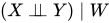$X\perp \!\!\!\perp Y$ neither implies nor is implied by $(X\perp \!\!\!\perp Y)\mid W$ .

First, suppose $W$ is 0 with probability 0.5 and 1 otherwise. When W = 0 take $X$ and $Y$ to be independent, each having the value 0 with probability 0.99 and the value 1 otherwise. When $W=1$ , $X$ and $Y$ are again independent, but this time they take the value 1 with probability 0.99. Then $(X\perp \!\!\!\perp Y)\mid W$ . But $X$ and $Y$ are dependent, because Pr(X = 0) < Pr(X = 0|Y = 0). This is because Pr(X = 0) = 0.5, but if Y = 0 then it's very likely that W = 0 and thus that X = 0 as well, so Pr(X = 0|Y = 0) > 0.5.

For the second example, suppose $X\perp \!\!\!\perp Y$ , each taking the values 0 and 1 with probability 0.5. Let $W$ be the product $X\cdot Y$ . Then when $W=0$ , Pr(X = 0) = 2/3, but Pr(X = 0|Y = 0) = 1/2, so $(X\perp \!\!\!\perp Y)\mid W$ is false. This is also an example of Explaining Away. See Kevin Murphy's tutorial where $X$ and $Y$ take the values "brainy" and "sporty".

03Conditional independence of random vectors

Two random vectors $\mathbf {X} =(X_{1},\ldots ,X_{l})^{\mathrm {T} }$ and $\mathbf {Y} =(Y_{1},\ldots ,Y_{m})^{\mathrm {T} }$ are conditionally independent given a third random vector $\mathbf {Z} =(Z_{1},\ldots ,Z_{n})^{\mathrm {T} }$ if and only if they are independent in their conditional cumulative distribution given $\mathbf {Z}$ . Formally:

$(\mathbf {X} \perp \!\!\!\perp \mathbf {Y} )\mid \mathbf {Z} \quad \iff \quad F_{\mathbf {X} ,\mathbf {Y} |\mathbf {Z} =\mathbf {z} }(\mathbf {x} ,\mathbf {y} )=F_{\mathbf {X} \,\mid \,\mathbf {Z} \,=\,\mathbf {z} }(\mathbf {x} )\cdot F_{\mathbf {Y} \,\mid \,\mathbf {Z} \,=\,\mathbf {z} }(\mathbf {y} )\quad {\text{for all }}\mathbf {x} ,\mathbf {y} ,\mathbf {z}$

Eq.3

where $\mathbf {x} =(x_{1},\ldots ,x_{l})^{\mathrm {T} }$ , $\mathbf {y} =(y_{1},\ldots ,y_{m})^{\mathrm {T} }$ and $\mathbf {z} =(z_{1},\ldots ,z_{n})^{\mathrm {T} }$ and the conditional cumulative distributions are defined as follows.

${\begin{aligned}F_{\mathbf {X} ,\mathbf {Y} \,\mid \,\mathbf {Z} \,=\,\mathbf {z} }(\mathbf {x} ,\mathbf {y} )&=\Pr(X_{1}\leq x_{1},\ldots ,X_{l}\leq x_{l},Y_{1}\leq y_{1},\ldots ,Y_{m}\leq y_{m}\mid Z_{1}=z_{1},\ldots ,Z_{n}=z_{n})\\[6pt]F_{\mathbf {X} \,\mid \,\mathbf {Z} \,=\,\mathbf {z} }(\mathbf {x} )&=\Pr(X_{1}\leq x_{1},\ldots ,X_{l}\leq x_{l}\mid Z_{1}=z_{1},\ldots ,Z_{n}=z_{n})\\[6pt]F_{\mathbf {Y} \,\mid \,\mathbf {Z} \,=\,\mathbf {z} }(\mathbf {y} )&=\Pr(Y_{1}\leq y_{1},\ldots ,Y_{m}\leq y_{m}\mid Z_{1}=z_{1},\ldots ,Z_{n}=z_{n})\end{aligned}}$

04Uses in Bayesian inference

Let p be the proportion of voters who will vote "yes" in an upcoming referendum. In taking an opinion poll, one chooses n voters randomly from the population. For i = 1, ..., n, let X_i = 1 or 0 corresponding, respectively, to whether or not the ith chosen voter will or will not vote "yes".

In a frequentist approach to statistical inference one would not attribute any probability distribution to p (unless the probabilities could be somehow interpreted as relative frequencies of occurrence of some event or as proportions of some population) and one would say that X₁, ..., X_n are independent random variables.

By contrast, in a Bayesian approach to statistical inference, one would assign a probability distribution to p regardless of the non-existence of any such "frequency" interpretation, and one would construe the probabilities as degrees of belief that p is in any interval to which a probability is assigned. In that model, the random variables X₁, ..., X_n are not independent, but they are conditionally independent given the value of p. In particular, if a large number of the Xs are observed to be equal to 1, that would imply a high conditional probability, given that observation, that p is near 1, and thus a high conditional probability, given that observation, that the next X to be observed will be equal to 1.

05Rules of conditional independence

A set of rules governing statements of conditional independence have been derived from the basic definition.

These rules were termed "Graphoid Axioms" by Pearl and Paz, because they hold in graphs, where $X\perp \!\!\!\perp A\mid B$ is interpreted to mean: "All paths from X to A are intercepted by the set B".

Symmetry

$X\perp \!\!\!\perp Y\mid Z\quad \Leftrightarrow \quad Y\perp \!\!\!\perp X\mid Z$

Proof:

From the definition of conditional independence,

$X\perp \!\!\!\perp Y\mid Z\quad \Leftrightarrow \quad P(X,Y\mid Z)=P(X\mid Z)P(Y\mid Z)\quad \Leftrightarrow \quad Y\perp \!\!\!\perp X\mid Z$

Decomposition

$X\perp \!\!\!\perp Y\mid Z\quad \Rightarrow \quad h(X)\perp \!\!\!\perp Y\mid Z$

Proof From the definition of conditional independence, we seek to show that:

$X\perp \!\!\!\perp Y\mid Z\quad \Rightarrow \quad P(h(X),Y\mid Z)=P(h(X)\mid Z)P(Y\mid Z)$

. The left side of this equality is:

$P(h(X)=a,Y=y\mid Z=z)=\sum _{X\colon h(X)=a}P(X=x,Y=y\mid Z=z)$

, where the expression on the right side of this equality is the summation over $X$ such that $h(X)=a$ of the conditional probability of $X,Y$ on $Z$ . Further decomposing,

${\begin{aligned}\sum _{X\colon h(X)=a}P(X=x,Y=y\mid Z=z)=&\sum _{X\colon h(X)=a}P(X=x\mid Z=z)P(Y=y\mid Z=z)\\=&P(Y=y\mid Z=z)\sum _{X\colon h(X)=a}P(X=x\mid Z=z)\\=&P(Y\mid Z)P(h(X)\mid Z)\end{aligned}}$

. Special cases of this property include

- Proof: Let us define $A=(X,W)$ and $h(\cdot )$ be an 'extraction' function $h(X,W)=X$ . Then:

${\begin{aligned}(X,W)\perp \!\!\!\perp Y\mid Z\quad &\Leftrightarrow \quad A\perp \!\!\!\perp Y\mid Z\\&\Rightarrow \quad h(A)\perp \!\!\!\perp Y\mid Z\quad &{\text{Decomposition}}\\&\Leftrightarrow \quad X\perp \!\!\!\perp Y\mid Z\end{aligned}}$

- Proof: Let us define $V=(Y,W)$ and $h(\cdot )$ be again an 'extraction' function $h(Y,W)=Y$ . Then:

${\begin{aligned}X\perp \!\!\!\perp (Y,W)\mid Z\quad &\Leftrightarrow \quad X\perp \!\!\!\perp V\mid Z\\&\Leftrightarrow \quad V\perp \!\!\!\perp X\mid Z\quad &{\text{Symmetry}}\\&\Rightarrow \quad h(V)\perp \!\!\!\perp X\mid Z\quad &{\text{Decomposition}}\\&\Leftrightarrow \quad Y\perp \!\!\!\perp X\mid Z\\&\Leftrightarrow \quad X\perp \!\!\!\perp Y\mid Z\quad &{\text{Symmetry}}\end{aligned}}$

Weak union

$X\perp \!\!\!\perp Y\mid Z\quad \Rightarrow \quad X\perp \!\!\!\perp Y\mid (Z,h(X))$

Proof:

Given $X\perp \!\!\!\perp Y\mid Z$ , we aim to show

${\begin{aligned}X\perp \!\!\!\perp Y\mid (Z,h(X))\quad &\Leftrightarrow \quad X\perp \!\!\!\perp Y\mid U\quad &{\text{where}}\quad U=(Z,h(X))\\&\Leftrightarrow \quad Y\perp \!\!\!\perp X\mid U\quad &{\text{Symmetry}}\\&\Leftrightarrow \quad P(Y\mid X,U)=P(Y\mid U)\\&\Leftrightarrow \quad P(Y\mid X,Z,h(X))=P(Y\mid Z,h(X))\end{aligned}}$

. We begin with the left side of the equation

${\begin{aligned}P(Y\mid X,Z,h(X))&=P(Y\mid X,Z)\\&=P(Y\mid Z)&{\text{Since by symmetry }}Y\perp \!\!\!\perp X\mid Z\end{aligned}}$

. From the given condition

${\begin{aligned}X\perp \!\!\!\perp Y\mid Z\quad &\Rightarrow \quad h(X)\perp \!\!\!\perp Y\mid Z\quad &{\text{Decomposition}}\\&\Leftrightarrow \quad Y\perp \!\!\!\perp h(X)\mid Z\quad &{\text{Symmetry}}\\&\Rightarrow \quad P(Y\mid Z,h(X))=P(Y\mid Z)\end{aligned}}$

. Thus $P(Y\mid X,Z,h(X))=P(Y\mid Z,h(X))$ , so we have shown that $X\perp \!\!\!\perp Y\mid (Z,h(X))$ .

Special Cases:

Some textbooks present the property as

$X\perp \!\!\!\perp (Y,W)\mid Z\quad \Rightarrow \quad X\perp \!\!\!\perp Y\mid (Z,W)$ .

$(X,W)\perp \!\!\!\perp Y\mid Z\quad \Rightarrow \quad X\perp \!\!\!\perp Y\mid (Z,W)$ .

Both versions can be shown to follow from the weak union property given initially via the same method as in the decomposition section above.

Contraction

$\left.{\begin{aligned}X\perp \!\!\!\perp A\mid B\\X\perp \!\!\!\perp B\end{aligned}}\right\}{\text{ and }}\quad \Rightarrow \quad X\perp \!\!\!\perp A,B$

Proof

This property can be proved by noticing $\Pr(X\mid A,B)=\Pr(X\mid B)=\Pr(X)$ , each equality of which is asserted by $X\perp \!\!\!\perp A\mid B$ and $X\perp \!\!\!\perp B$ , respectively.

Intersection

For strictly positive probability distributions, the following also holds:

$\left.{\begin{aligned}X\perp \!\!\!\perp Y\mid Z,W\\X\perp \!\!\!\perp W\mid Z,Y\end{aligned}}\right\}{\text{ and }}\quad \Rightarrow \quad X\perp \!\!\!\perp W,Y\mid Z$

Proof

By assumption:

Using this equality, together with the Law of total probability applied to $P(X|Z)$ :

${\begin{aligned}P(X|Z)&=\sum _{w\in W}P(X|Z,W=w)P(W=w|Z)\\[4pt]&=\sum _{w\in W}P(X|Y,Z)P(W=w|Z)\\[4pt]&=P(X|Z,Y)\sum _{w\in W}P(W=w|Z)\\[4pt]&=P(X|Z,Y)\end{aligned}}$

Technical note: since these implications hold for any probability space, they will still hold if one considers a sub-universe by conditioning everything on another variable, say K. For example, $X\perp \!\!\!\perp Y\Rightarrow Y\perp \!\!\!\perp X$ would also mean that $X\perp \!\!\!\perp Y\mid K\Rightarrow Y\perp \!\!\!\perp X\mid K$ .

Watch videos about Conditional independenceExplainers and documentaries on YouTube (opens in a new tab)

Sources and credits

This article is adapted from the Wikipedia article “Conditional independence”, written by its contributors and licensed under CC BY-SA 4.0. Fathomly has changed the layout, removed citation markers, navigation and maintenance notices, and adjusted punctuation. This adapted version is shared under the same license. For references, see the original article.

Images, from Wikimedia Commons:

Standard deviation diagram micro.svg by Ainali, CC BY-SA 3.0

Fathomly is not affiliated with or endorsed by the Wikimedia Foundation. Spotted a problem? Tell us.