Compound Poisson process
Random process in probability theory
A compound Poisson process is a continuous-time stochastic process with jumps. The jumps arrive randomly according to a Poisson process and the size of the jumps is also random, with a specified probability distribution. To be precise, a compound Poisson process, parameterised by a rate 

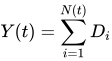
where, 

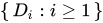

When 
01Properties of the compound Poisson process
The expected value of a compound Poisson process can be calculated using a result known as Wald's equation as:

Making similar use of the law of total variance, the variance can be calculated as:
![{\begin{aligned}\operatorname {var} (Y(t))&=\operatorname {E} (\operatorname {var} (Y(t)\mid N(t)))+\operatorname {var} (\operatorname {E} (Y(t)\mid N(t)))\\[5pt]&=\operatorname {E} (N(t)\operatorname {var} (D))+\operatorname {var} (N(t)\operatorname {E} (D))\\[5pt]&=\operatorname {var} (D)\operatorname {E} (N(t))+\operatorname {E} (D)^{2}\operatorname {var} (N(t))\\[5pt]&=\operatorname {var} (D)\lambda t+\operatorname {E} (D)^{2}\lambda t\\[5pt]&=\lambda t(\operatorname {var} (D)+\operatorname {E} (D)^{2})\\[5pt]&=\lambda t\operatorname {E} (D^{2}).\end{aligned}}](https://wikimedia.org/api/rest_v1/media/math/render/svg/5a818cc242b7003a3d5f043f431fdf57801e9734)
Lastly, using the law of total probability, the moment generating function can be given as follows:

![{\begin{aligned}\operatorname {E} (e^{sY})&=\sum _{i}e^{si}\Pr(Y(t)=i)\\[5pt]&=\sum _{i}e^{si}\sum _{n}\Pr(Y(t)=i\mid N(t)=n)\Pr(N(t)=n)\\[5pt]&=\sum _{n}\Pr(N(t)=n)\sum _{i}e^{si}\Pr(Y(t)=i\mid N(t)=n)\\[5pt]&=\sum _{n}\Pr(N(t)=n)\sum _{i}e^{si}\Pr(D_{1}+D_{2}+\cdots +D_{n}=i)\\[5pt]&=\sum _{n}\Pr(N(t)=n)M_{D}(s)^{n}\\[5pt]&=\sum _{n}\Pr(N(t)=n)e^{n\ln(M_{D}(s))}\\[5pt]&=M_{N(t)}(\ln(M_{D}(s)))\\[5pt]&=e^{\lambda t\left(M_{D}(s)-1\right)}.\end{aligned}}](https://wikimedia.org/api/rest_v1/media/math/render/svg/5b8480ad2cecd8cd45d38ad108824ed88fda17cc)
02Exponentiation of measures
Let N, Y, and D be as above. Let μ be the probability measure according to which D is distributed, i.e.

Let δ0 be the trivial probability distribution putting all of the mass at zero. Then the probability distribution of Y(t) is the measure

where the exponential exp(ν) of a finite measure ν on Borel subsets of the real line is defined by
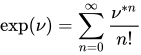
and
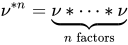
is a convolution of measures, and the series converges weakly.
Sources and credits
This article is adapted from the Wikipedia article “Compound Poisson process”, written by its contributors and licensed under CC BY-SA 4.0. Fathomly has changed the layout, removed citation markers, navigation and maintenance notices, and adjusted punctuation. This adapted version is shared under the same license. For references, see the original article.
Fathomly is not affiliated with or endorsed by the Wikimedia Foundation. Spotted a problem? Tell us.

