Branch and bound

The goal of a branch-and-bound algorithm is to find a value x that maximizes or minimizes the value of a real-valued function f(x), called an objective function, among some set S of admissible or candidate solutions. The set S is called the search space, or feasible region. The rest of this section assumes that minimization of f(x) is desired; this assumption comes without loss of generality, since one can find the maximum value of f(x) by finding the minimum of g(x) = −f(x). A B&B algorithm operates according to two principles:

• It recursively splits the search space into smaller spaces, then minimizes f(x) on these smaller spaces; the splitting is called branching.
• Branching alone would amount to brute-force enumeration of candidate solutions and testing them all. To improve on the performance of brute-force search, a B&B algorithm keeps track of bounds on the minimum that it is trying to find, and uses these bounds to "prune" the search space, eliminating candidate solutions that it can prove will not contain an optimal solution.

Turning these principles into a concrete algorithm for a specific optimization problem requires some kind of data structure that represents sets of candidate solutions. Such a representation is called an instance of the problem. Denote the set of candidate solutions of an instance I by S_I. The instance representation has to come with three operations:

• branch(I) produces two or more instances that each represent a subset of S_I. (Typically, the subsets are disjoint to prevent the algorithm from visiting the same candidate solution twice, but this is not required. However, an optimal solution among S_I must be contained in at least one of the subsets.)
• bound(I) computes a lower bound on the value of any candidate solution in the space represented by I, that is, bound(I) ≤ f(x) for all x in S_I.
• solution(I) determines whether I represents a single candidate solution. (Optionally, if it does not, then the operation may choose to return some feasible solution from among S_I.) If solution(I) returns a solution, then f(solution(I)) provides an upper bound for the optimal objective value over the whole space of feasible solutions.

Using these operations, a B&B algorithm performs a top-down recursive search through the tree of instances formed by the branch operation. Upon visiting an instance I, it checks whether bound(I) is equal to or greater than the current upper bound; if so, I may be safely discarded from the search and the recursion stops. This pruning step is usually implemented by maintaining a global variable that records the minimum upper bound seen among all instances examined so far.

Generic version

The following is the skeleton of a generic branch-and-bound algorithm for minimizing an arbitrary objective function f. To obtain an actual algorithm from this, one requires a bounding function bound, that computes lower bounds of f on nodes of the search tree, as well as a problem-specific branching rule.

1. Using a heuristic, find a solution x_h to the optimization problem. Store its value, B = f(x_h). (If no heuristic is available, set B to infinity.) B will denote the best solution found so far, and will be used as an upper bound on candidate solutions.
2. Initialize a queue to hold a partial solution with none of the variables of the problem assigned.
3. Loop until the queue is empty:
   1. Take a node N off the queue.
   2. If N represents a single candidate solution x and f(x) < B, then x is the best solution so far. Record it and set B ← f(x). The same can be done with a heuristic whenever the node does not identify a unique solution.
   3. Else, branch on N to produce new nodes N_i. Add all feasible nodes for which bound(N_i) < B to the queue. The remaining nodes, having a lower bound greater than or equal to the upper bound of the problem, will never lead to the optimal solution and are discarded.

Several different queue data structures can be used. A stack (LIFO queue) will yield a depth-first algorithm. A best-first branch-and-bound algorithm can be obtained by using a priority queue that sorts nodes on their lower bounds. The depth-first variant is recommended when no good heuristic is available for producing an initial solution, because it quickly produces full solutions, and therefore upper bounds.

Improvements

When is a vector of , branch-and-bound algorithms can be combined with interval analysis and contractor techniques to provide guaranteed enclosures of the global minimum.

This approach is used for a number of NP-hard problems:

• Integer programming
• Nonlinear programming
• Travelling salesman problem (TSP)
• Quadratic assignment problem (QAP)
• Maximum satisfiability problem (MAX-SAT)
• Nearest neighbor search (by Keinosuke Fukunaga)
• Flow shop scheduling
• Cutting stock problem
• Computational phylogenetics
• Set inversion
• Parameter estimation
• 0/1 knapsack problem
• Set cover problem
• Feature selection in machine learning
• Structured prediction in computer vision
• Arc routing problem, including the Chinese Postman problem
• Talent Scheduling, scenes-shooting arrangement problem

Branch-and-bound may also be a base of various heuristics. For example, one may wish to stop branching when the gap between the upper and lower bounds becomes smaller than a certain threshold. This is used when the solution is "good enough for practical purposes" and can greatly reduce the computations required. This type of solution is particularly applicable when the cost function used is noisy or is the result of statistical estimates and so is not known precisely but rather only known to lie within a range of values with a specific probability.

Nau et al. present a generalization of branch and bound that also subsumes the A*, B* and alpha-beta search algorithms.

Branch-and-bound can be used to maximize with the constraints

and are integers.

The first step is to relax the integer constraint. We have two extreme points for the first equation that form a line: 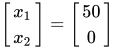and . We can form the second line with the vector points and .

The third point is . This is a convex hull region, so the solution lies on one of the vertices of the region. We can find the intersection using row reduction, which is with a value of 276 + 2/3. We test the other endpoints by sweeping the line over the region and find this is the maximum over the reals.

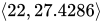
We choose the variable with the maximum fractional part, in this case becomes the parameter for the branch and bound method. We branch to and obtain 276 at . We have reached an integer solution so we move to the other branch . We obtain 275.75 at . We have a decimal, so we branch to and we find 274.571 at . We try the other branch and there are no feasible solutions. Therefore, the maximum is 276 with and .