Encyclopedia

Binomial distribution

Probability distribution

Wikipedia contributorsAdapted for Fathomly · View authors

15 min read
Source updated September 11, 2026

In probability theory and statistics, the binomial distribution with parameters n and p is the discrete probability distribution of the number of successes in a sequence of n independent experiments, each asking a yes-no question, and each with its own Boolean-valued outcome: success (with probability p) or failure (with probability q = 1 − p). A single success/failure experiment is also called a Bernoulli trial or Bernoulli experiment, and a sequence of outcomes is called a Bernoulli process. For a single trial, that is, when n = 1, the binomial distribution is a Bernoulli distribution. The binomial distribution is the basis for the binomial test of statistical significance.

The binomial distribution is frequently used to model the number of successes in a sample of size n drawn with replacement from a population of size N. If the sampling is carried out without replacement, the draws are not independent and so the resulting distribution is a hypergeometric distribution, not a binomial one. However, for N much larger than n, the binomial distribution remains a good approximation, and is widely used.

01Definitions

Probability mass function

If the random variable X follows the binomial distribution with parameters $n\in \mathbb {N}$ (a natural number) and p ∈ [0, 1], we write X ~ B(n, p). The probability of getting exactly k successes in n independent Bernoulli trials (with the same rate p) is given by the probability mass function: $f(k,n,p)=\Pr(X=k)={\binom {n}{k}}p^{k}(1-p)^{n-k}$ for k = 0, 1, 2, ..., n, where ${\binom {n}{k}}={\frac {n!}{k!(n-k)!}}$ is the binomial coefficient. The formula can be understood as follows: p^k q^n−k is the probability of obtaining the sequence of n independent Bernoulli trials in which k trials are "successes" and the remaining n − k trials are "failures". Since the trials are independent with probabilities remaining constant between them, any sequence of n trials with k successes (and n − k failures) has the same probability of being achieved (regardless of positions of successes within the sequence). There are ${\textstyle {\binom {n}{k}}$ such sequences, since the binomial coefficient ${\textstyle {\binom {n}{k}}$ counts the number of ways to choose the positions of the k successes among the n trials. The binomial distribution is concerned with the probability of obtaining any of these sequences, meaning the probability of obtaining one of them (p^k q^n−k) must be added ${\textstyle {\binom {n}{k}}$ times, hence ⁠ $\textstyle \Pr(X=k)={\binom {n}{k}}p^{k}(1-p)^{n-k}$ ⁠.

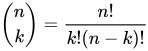
In creating reference tables for binomial distribution probability, usually, the table is filled in up to ⁠ $\textstyle {\tfrac {n}{2}}$ ⁠ values. This is because for ⁠ $\textstyle k>{\tfrac {n}{2}}$ ⁠, the probability can be calculated by its complement as $f(k,n,p)=f(n-k,n,1-p).$

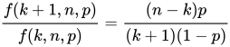
Looking at the expression f(k, n, p) as a function of k, there is a k value that maximizes it. This k value can be found by calculating ${\frac {f(k+1,n,p)}{f(k,n,p)}}={\frac {(n-k)p}{(k+1)(1-p)}}$ and comparing it to 1. There is always an integer M that satisfies $(n+1)p-1\leq M<(n+1)p.$

f(k, n, p) is monotone increasing for k < M and monotone decreasing for k > M, with the exception of the case where (n + 1)p is an integer. In this case, there are two values for which f is maximal: (n + 1)p and (n + 1)p − 1. M is the most probable outcome (that is, the most likely, although this can still be unlikely overall) of the Bernoulli trials and is called the mode.

Example

Suppose a biased coin comes up heads with probability 0.3 when tossed. The probability of seeing exactly 4 heads in 6 tosses is $f(4,6,0.3)={\binom {6}{4}}0.3^{4}(1-0.3)^{6-4}=0.059535.$

Cumulative distribution function

The cumulative distribution function can be expressed as: $F(k;n,p)=\Pr(X\leq k)=\sum _{i=0}^{\lfloor k\rfloor }{n \choose i}p^{i}(1-p)^{n-i},$ where $\lfloor k\rfloor$ is the "floor" under k; that is, the greatest integer less than or equal to k.

It can also be represented in terms of the regularized incomplete beta function, as follows: ${\begin{aligned}F(k;n,p)&=\Pr(X\leq k)\\&=I_{1-p}(n-k,k+1)\\&=(n-k){n \choose k}\int _{0}^{1-p}t^{n-k-1}(1-t)^{k}\,dt,\end{aligned}}$ which is equivalent to the cumulative distribution functions of the beta distribution and of the F-distribution: $F(k;n,p)=F_{\text{beta-distribution}}\left(x=1-p;\alpha =n-k,\beta =k+1\right)$ $F(k;n,p)=F_{F{\text{-distribution}}}\left(x={\frac {1-p}{p}}{\frac {k+1}{n-k}};d_{1}=2(n-k),d_{2}=2(k+1)\right).$

Some closed-form bounds for the cumulative distribution function are given below.

02Properties

Expected value and variance

If X ~ B(n, p), that is, X is a binomially distributed random variable, n being the total number of experiments and p the probability of each experiment yielding a successful result, then the expected value of X is: $\operatorname {E} [X]=np.$

This follows from the linearity of the expected value along with the fact that X is the sum of n identical Bernoulli random variables, each with expected value p. In other words, if $X_{1},\ldots ,X_{n}$ are identical (and independent) Bernoulli random variables with parameter p, then X = X₁ + ... + X_n and $\operatorname {E} [X]=\operatorname {E} [X_{1}+\cdots +X_{n}]=\operatorname {E} [X_{1}]+\cdots +\operatorname {E} [X_{n}]=p+\cdots +p=np.$

The variance is: $\operatorname {Var} (X)=npq=np(1-p).$

This similarly follows from the fact that the variance of a sum of independent random variables is the sum of the variances.

Higher moments

The first 6 central moments, defined as $\mu _{c}=\operatorname {E} \left[(X-\operatorname {E} [X])^{c}\right]$ , are given by ${\begin{aligned}\mu _{1}&=0,\\\mu _{2}&=np\left(1-p\right),\\\mu _{3}&=np\left(1-p\right)\left(1-2p\right),\\\mu _{4}&=np\left(1-p\right)\left[1+\left(3n-6\right)p\left(1-p\right)\right],\\\mu _{5}&=np\left(1-p\right)\left(1-2p\right)\left[1+\left(10n-12\right)p\left(1-p\right)\right],\\\mu _{6}&=np\left(1-p\right)\left[1-30p\left(1-p\right)\left[1-4p(1-p)\right]+5np\left(1-p\right)\left[5-26p\left(1-p\right)\right]+15n^{2}p^{2}\left(1-p\right)^{2}\right].\end{aligned}}$

The non-central moments satisfy ${\begin{aligned}\operatorname {E} [X]&=np,\\\operatorname {E} [X^{2}]&=np(1-p)+n^{2}p^{2},\end{aligned}}$ and in general $\operatorname {E} [X^{c}]=\sum _{k=0}^{c}\left\{{c \atop k}\right\}n^{\underline {k}}p^{k},$ where ${\textstyle \left\{{c \atop k}\right\}$ are the Stirling numbers of the second kind, and $n^{\underline {k}}=n(n-1)\cdots (n-k+1)$ is the $k$ -th falling power of $n$ . A simple bound follows by bounding the Binomial moments via the higher Poisson moments: $\operatorname {E} [X^{c}]\leq \left[{\frac {c}{\ln \left(1+{\frac {c}{np}}\right)}}\right]^{c}\leq (np)^{c}\exp \left({\frac {c^{2}}{2np}}\right).$ This shows that if $c=O({\sqrt {np}})$ , then $\operatorname {E} [X^{c}]$ is at most a constant factor away from $\operatorname {E} [X]^{c}$ .

The moment-generating function is $M_{X}(t)=\mathbb {E} [e^{tX}]=(1-p+pe^{t})^{n}$ .

Mode

Usually the mode of a binomial B(n, p) distribution is equal to $\lfloor (n+1)p\rfloor$ , where $\lfloor \cdot \rfloor$ is the floor function. However, when (n + 1)p is an integer and p is neither 0 nor 1, then the distribution has two modes: (n + 1)p and (n + 1)p − 1. When p is equal to 0 or 1, the mode will be 0 and n correspondingly. These cases can be summarized as follows: ${\text{mode}}={\begin{cases}\lfloor (n+1)\,p\rfloor &{\text{if }}(n+1)p{\text{ is 0 or a noninteger}},\\(n+1)\,p\ {\text{ and }}\ (n+1)\,p-1&{\text{if }}(n+1)p\in \{1,\dots ,n\},\\n&{\text{if }}(n+1)p=n+1.\end{cases}}$

Proof: Let $f(k)={\binom {n}{k}}p^{k}q^{n-k}.$

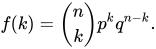
For $p=0$ only $f(0)$ has a nonzero value with $f(0)=1$ . For $p=1$ we find $f(n)=1$ and $f(k)=0$ for $k\neq n$ . This proves that the mode is 0 for $p=0$ and $n$ for $p=1$ .

Let $0<p<1$ . We find ${\frac {f(k+1)}{f(k)}}={\frac {(n-k)p}{(k+1)(1-p)}}.$

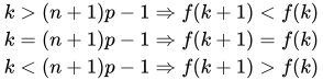
From this follows ${\begin{aligned}k>(n+1)p-1\Rightarrow f(k+1)<f(k)\\k=(n+1)p-1\Rightarrow f(k+1)=f(k)\\k<(n+1)p-1\Rightarrow f(k+1)>f(k)\end{aligned}}$

So when $(n+1)p-1$ is an integer, then $(n+1)p-1$ and $(n+1)p$ is a mode. In the case that $(n+1)p-1\notin \mathbb {Z}$ , then only $\lfloor (n+1)p-1\rfloor +1=\lfloor (n+1)p\rfloor$ is a mode.

Median

In general, there is no single formula to find the median for a binomial distribution, and it may even be non-unique. However, several special results have been established:

If np is an integer, then the mean, median, and mode coincide and equal np.
Any median m must lie within the interval $\lfloor np\rfloor \leq m\leq \lceil np\rceil$ .
A median m cannot lie too far away from the mean: $|m-np|\leq \min\{{\ln 2},\max\{p,1-p\}\}$ .
The median is unique and equal to m = round(np) when |m − np| ≤ min{p, 1 − p} (except for the case when p = 1/2 and n is odd).
When p is a rational number (with the exception of p = 1/2 and n odd), the median is unique.
When ${\textstyle p={\tfrac {1}{2}}$ and n is odd, any number m in the interval ${\textstyle {\frac {1}{2}}\left(n-1\right)\leq m\leq {\frac {1}{2}}\left(n+1\right)$ is a median of the binomial distribution. If ${\textstyle p={\tfrac {1}{2}}$ and n is even, then ${\textstyle m={\tfrac {n}{2}}$ is the unique median.

Tail bounds

For k ≤ np, upper bounds can be derived for the lower tail of the cumulative distribution function $F(k;n,p)=\Pr(X\leq k)$ , the probability that there are at most k successes. Since $\Pr(X\geq k)=F(n-k;n,1-p)$ , these bounds can also be seen as bounds for the upper tail of the cumulative distribution function for k ≥ np.

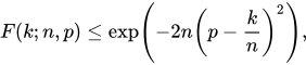
Hoeffding's inequality yields the simple bound $F(k;n,p)\leq \exp \left(-2n\left(p-{\frac {k}{n}}\right)^{2}\right),\!$ which is however not very tight. In particular, for p = 1, we have that F(k; n, p) = 0 (for fixed k, n with k < n), but Hoeffding's bound evaluates to a positive constant.

A sharper bound can be obtained from the Chernoff bound: $F(k;n,p)\leq \exp \left(-nD{\left({\frac {k}{n}}\parallel p\right)}\right)$ where D(a ∥ p) is the relative entropy (or Kullback-Leibler divergence) between an a-coin and a p-coin (that is, between the Bernoulli(a) and Bernoulli(p) distribution): $D(a\parallel p)=(a)\ln {\frac {a}{p}}+(1-a)\ln {\frac {1-a}{1-p}}.\!$

Asymptotically, this bound is reasonably tight; see for details.

One can also obtain lower bounds on the tail F(k; n, p), known as anti-concentration bounds. By approximating the binomial coefficient with Stirling's formula it can be shown that $F(k;n,p)\geq {\frac {1}{\sqrt {8n{\tfrac {k}{n}}(1-{\tfrac {k}{n}})}}}\exp \left(-nD{\left({\frac {k}{n}}\parallel p\right)}\right),$ which implies the simpler but looser bound $F(k;n,p)\geq {\frac {1}{\sqrt {2n}}}\exp \left(-nD\left({\frac {k}{n}}\parallel p\right)\right).$

For p = 1/2 and k ≥ 3n/8 for even n, it is possible to make the denominator constant: $F(k;n,{\tfrac {1}{2}})\geq {\frac {1}{15}}\exp \left(-16n\left({\frac {1}{2}}-{\frac {k}{n}}\right)^{2}\right).\!$

03Statistical inference

Estimation of parameters

When n is known, the parameter p can be estimated using the proportion of successes: ${\widehat {p}}={\frac {x}{n}}.$ This estimator is found using maximum likelihood estimator and also the method of moments. This estimator is unbiased and uniformly with minimum variance, proven using Lehmann-Scheffé theorem, since it is based on a minimal sufficient and complete statistic (that is, x). It is also consistent both in probability and in MSE. This statistic is asymptotically normal thanks to the central limit theorem, because it is the same as taking the mean over Bernoulli samples. It has a variance of $\operatorname {Var} ({\hat {p}})={\frac {p(1-p)}{n}}$ , a property which is used in various ways, such as in Wald's confidence intervals.

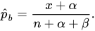
A closed form Bayes estimator for p also exists when using the Beta distribution as a conjugate prior distribution. When using a general $\operatorname {Beta} (\alpha ,\beta )$ as a prior, the posterior mean estimator is: ${\widehat {p}}_{b}={\frac {x+\alpha }{n+\alpha +\beta }}.$ The Bayes estimator is asymptotically efficient and as the sample size approaches infinity (n → ∞), it approaches the MLE solution. The Bayes estimator is biased (how much depends on the priors), admissible and consistent in probability. Using the Bayesian estimator with the Beta distribution can be used with Thompson sampling.

For the special case of using the standard uniform distribution as a non-informative prior, $\operatorname {Beta} (\alpha {=}1,\,\beta {=}1)=U(0,1)$ , the posterior mean estimator becomes: ${\widehat {p}}_{b}={\frac {x+1}{n+2}}.$ (A posterior mode should just lead to the standard estimator.) This method is called the rule of succession, which was introduced in the 18th century by Pierre-Simon Laplace.

When relying on Jeffreys prior, the prior is ${\textstyle \operatorname {Beta} (\alpha {=}{\tfrac {1}{2}},\,\beta {=}{\tfrac {1}{2}})$ , which leads to the estimator: ${\widehat {p}}_{\mathrm {Jeffreys} }={\frac {x+{\frac {1}{2}}}{n+1}}.$

When estimating p with very rare events and a small n (for example, if x = 0), then using the standard estimator leads to ${\widehat {p}}=0,$ which sometimes is unrealistic and undesirable. In such cases there are various alternative estimators. One way is to use the Bayes estimator ${\widehat {p}}_{b}$ , leading to: ${\widehat {p}}_{b}={\frac {1}{n+2}}.$ Another method is to use the upper bound of the confidence interval obtained using the rule of three: ${\widehat {p}}_{\text{rule of 3}}={\frac {3}{n}}.$

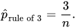
Confidence intervals for the parameter p

Even for quite large values of n, the actual distribution of the mean is significantly nonnormal. Because of this problem several methods to estimate confidence intervals have been proposed.

In the equations for confidence intervals below, the variables have the following meaning:

n₁ is the number of successes out of n, the total number of trials
${\widehat {p\,}}={\frac {n_{1}}{n}}$ is the proportion of successes
$z$ is the $1-{\tfrac {1}{2}}\alpha$ quantile of a standard normal distribution (that is, probit) corresponding to the target error rate $\alpha$ . For example, for a 95% confidence level the error $\alpha =0.05$ , so $1-{\tfrac {1}{2}}\alpha =0.975$ and $z=1.96$ .

Wald method

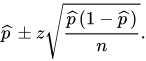
${\widehat {p\,}}\pm z{\sqrt {\frac {{\widehat {p\,}}(1-{\widehat {p\,}})}{n}}}.$

A continuity correction of 0.5 / n may be added.

Agresti-Coull method

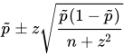
${\tilde {p}}\pm z{\sqrt {\frac {{\tilde {p}}(1-{\tilde {p}})}{n+z^{2}}}}$

Here the estimate of p is modified to ${\tilde {p}}={\frac {n_{1}+{\frac {1}{2}}z^{2}}{n+z^{2}}}$

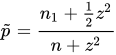
This method works well for n > 10 and n₁ ≠ 0, n. See here for $n\leq 10$ . For n₁ = 0, n use the Wilson (score) method below.

Arcsine method

$\sin ^{2}\left(\arcsin \left({\sqrt {\hat {p}}}\right)\pm {\frac {z}{2{\sqrt {n}}}}\right).$

Wilson (score) method

The notation in the formula below differs from the previous formulas in two respects:

Firstly, z_x has a slightly different interpretation in the formula below: it has its ordinary meaning of 'the xth quantile of the standard normal distribution', rather than being a shorthand for 'the (1 − x)th quantile'.
Secondly, this formula does not use a plus-minus to define the two bounds. Instead, one may use $z=z_{\alpha /2}$ to get the lower bound, or use $z=z_{1-\alpha /2}$ to get the upper bound. For example: for a 95% confidence level the error $\alpha =0.05$ , so one gets the lower bound by using $z=z_{\alpha /2}=z_{0.025}=-1.96$ , and one gets the upper bound by using $z=z_{1-\alpha /2}=z_{0.975}=1.96$ .

${\frac {{\hat {p}}+{\frac {z^{2}}{2n}}+z{\sqrt {{\frac {{\hat {p}}\left(1-{\hat {p}}\right)}{n}}+{\frac {z^{2}}{4n^{2}}}}}}{1+{\frac {z^{2}}{n}}}}$

Comparison

The so-called "exact" (Clopper-Pearson) method is the most conservative. (Exact does not mean perfectly accurate; rather, it indicates that the estimates will not be less conservative than the true value.)

The Wald method, although commonly recommended in textbooks, is the most biased.

04Related distributions

Sums of binomials

If X ~ B(n, p) and Y ~ B(m, p) are independent binomial variables with the same probability p, then X + Y is again a binomial variable; its distribution is Z = X + Y ~ B(n + m, p): ${\begin{aligned}\operatorname {P} (Z=k)&=\sum _{i=0}^{k}\left[{\binom {n}{i}}p^{i}(1-p)^{n-i}\right]\left[{\binom {m}{k-i}}p^{k-i}(1-p)^{m-k+i}\right]\\&={\binom {n+m}{k}}p^{k}(1-p)^{n+m-k}\end{aligned}}$

A Binomial distributed random variable X ~ B(n, p) can be considered as the sum of n Bernoulli distributed random variables. So the sum of two Binomial distributed random variables X ~ B(n, p) and Y ~ B(m, p) is equivalent to the sum of n + m Bernoulli distributed random variables, which means Z = X + Y ~ B(n + m, p). This can also be proven directly using the addition rule.

However, if X and Y do not have the same probability p, then the variance of the sum will be smaller than the variance of a binomial variable distributed as B(n + m, p).

Poisson binomial distribution

The binomial distribution is a special case of the Poisson binomial distribution, which is the distribution of a sum of n independent non-identical Bernoulli trials B(p_i).

Ratio of two binomial distributions

This result was first derived by Katz and coauthors in 1978.

Let X ~ B(n, p₁) and Y ~ B(m, p₂) be independent. Let T = (X/n) / (Y/m).

Then log(T) is approximately normally distributed with mean log(p₁/p₂) and variance ((1/p₁) − 1)/n + ((1/p₂) − 1)/m.

Conditional binomials

If X ~ B(n, p) and Y | X ~ B(X, q) (the conditional distribution of Y, given X), then Y is a simple binomial random variable with distribution Y ~ B(n, pq).

For example, imagine throwing n balls to a basket U_X and taking the balls that hit and throwing them to another basket U_Y. If p is the probability to hit U_X then X ~ B(n, p) is the number of balls that hit U_X. If q is the probability to hit U_Y then the number of balls that hit U_Y is Y ~ B(X, q) and therefore Y ~ B(n, pq).

[Proof]

Since $X\sim \mathrm {B} (n,p)$ and $Y\sim \mathrm {B} (X,q)$ , by the law of total probability, ${\begin{aligned}\Pr[Y=m]&=\sum _{k=m}^{n}\Pr[Y=m\mid X=k]\Pr[X=k]\\[2pt]&=\sum _{k=m}^{n}{\binom {n}{k}}{\binom {k}{m}}p^{k}q^{m}(1-p)^{n-k}(1-q)^{k-m}\end{aligned}}$ Since ${\tbinom {n}{k}}{\tbinom {k}{m}}={\tbinom {n}{m}}{\tbinom {n-m}{k-m}},$ the equation above can be expressed as $\Pr[Y=m]=\sum _{k=m}^{n}{\binom {n}{m}}{\binom {n-m}{k-m}}p^{k}q^{m}(1-p)^{n-k}(1-q)^{k-m}$ Factoring $p^{k}=p^{m}p^{k-m}$ and pulling all the terms that don't depend on $k$ out of the sum now yields ${\begin{aligned}\Pr[Y=m]&={\binom {n}{m}}p^{m}q^{m}\left(\sum _{k=m}^{n}{\binom {n-m}{k-m}}p^{k-m}(1-p)^{n-k}(1-q)^{k-m}\right)\\[2pt]&={\binom {n}{m}}(pq)^{m}\left(\sum _{k=m}^{n}{\binom {n-m}{k-m}}\left(p(1-q)\right)^{k-m}(1-p)^{n-k}\right)\end{aligned}}$ After substituting $i=k-m$ in the expression above, we get $\Pr[Y=m]={\binom {n}{m}}(pq)^{m}\left(\sum _{i=0}^{n-m}{\binom {n-m}{i}}(p-pq)^{i}(1-p)^{n-m-i}\right)$ Notice that the sum (in the parentheses) above equals $(p-pq+1-p)^{n-m}$ by the binomial theorem. Substituting this in finally yields ${\begin{aligned}\Pr[Y=m]&={\binom {n}{m}}(pq)^{m}(p-pq+1-p)^{n-m}\\[4pt]&={\binom {n}{m}}(pq)^{m}(1-pq)^{n-m}\end{aligned}}$ and thus $Y\sim \mathrm {B} (n,pq)$ as desired.

Bernoulli distribution

The Bernoulli distribution is a special case of the binomial distribution, where n = 1. Symbolically, X ~ B(1, p) has the same meaning as X ~ Bernoulli(p). Conversely, any binomial distribution, B(n, p), is the distribution of the sum of n independent Bernoulli trials, Bernoulli(p), each with the same probability p.

Normal approximation

If n is large enough, then the skew of the distribution is not too great. In this case a reasonable approximation to B(n, p) is given by the normal distribution ${\mathcal {N}}(np,\,np(1-p)),$ and this basic approximation can be improved in a simple way by using a suitable continuity correction. The basic approximation generally improves as n increases (at least 20) and is better when p is not near to 0 or 1. Various rules of thumb may be used to decide whether n is large enough, and p is far enough from the extremes of zero or one:

One rule is that for n > 5 the normal approximation is adequate if the absolute value of the skewness is strictly less than 0.3; that is, if ${\frac {|1-2p|}{\sqrt {np(1-p)}}}={\frac {1}{\sqrt {n}}}\left|{\sqrt {\frac {1-p}{p}}}-{\sqrt {\frac {p}{1-p}}}\,\right|<0.3.$

This can be made precise using the Berry-Esseen theorem.

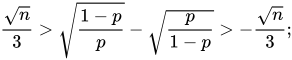
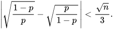
A stronger rule states that the normal approximation is appropriate only if everything within 3 standard deviations of its mean is within the range of possible values; that is, only if $\mu \pm 3\sigma =np\pm 3{\sqrt {np(1-p)}}\in (0,n).$

This 3-standard-deviation rule is equivalent to the following conditions, which also imply the first rule above.

n>9\left({\frac {1-p}{p}}\right)\quad {\text{and}}\quad n>9\left({\frac {p}{1-p}}\right).

[Proof]

The rule $np\pm 3{\sqrt {np(1-p)}}\in (0,n)$ is totally equivalent to request that $np-3{\sqrt {np(1-p)}}>0\quad {\text{and}}\quad np+3{\sqrt {np(1-p)}}<n.$ Moving terms around yields: $np>3{\sqrt {np(1-p)}}\quad {\text{and}}\quad n(1-p)>3{\sqrt {np(1-p)}}.$ Since $0<p<1$ , we can apply the square power and divide by the respective factors $np^{2}$ and $n(1-p)^{2}$ , to obtain the desired conditions: $n>9\left({\frac {1-p}{p}}\right)\quad {\text{and}}\quad n>9\left({\frac {p}{1-p}}\right).$ Notice that these conditions automatically imply that $n>9$ . On the other hand, apply again the square root and divide by 3, ${\frac {\sqrt {n}}{3}}>{\sqrt {\frac {1-p}{p}}}>0\quad {\text{and}}\quad {\frac {\sqrt {n}}{3}}>{\sqrt {\frac {p}{1-p}}}>0.$ Subtracting the second set of inequalities from the first one yields: ${\frac {\sqrt {n}}{3}}>{\sqrt {\frac {1-p}{p}}}-{\sqrt {\frac {p}{1-p}}}>-{\frac {\sqrt {n}}{3}};$ and so, the desired first rule is satisfied, $\left|{\sqrt {\frac {1-p}{p}}}-{\sqrt {\frac {p}{1-p}}}\,\right|<{\frac {\sqrt {n}}{3}}.$

Another commonly used rule is that both values np and n(1 − p) must be greater than or equal to 5. However, the specific number varies from source to source, and depends on how good an approximation one wants. In particular, if one uses 9 instead of 5, the rule implies the results stated in the previous paragraphs.

[Proof]

Assume that both values $np$ and $n(1-p)$ are greater than 9. Since $0<p<1$ , we easily have that $np\geq 9>9(1-p)\quad {\text{and}}\quad n(1-p)\geq 9>9p.$ We only have to divide now by the respective factors $p$ and $1-p$ , to deduce the alternative form of the 3-standard-deviation rule: $n>9\left({\frac {1-p}{p}}\right)\quad {\text{and}}\quad n>9\left({\frac {p}{1-p}}\right).$

The following is an example of applying a continuity correction. Suppose one wishes to calculate Pr(X ≤ 8) for a binomial random variable X. If Y has a distribution given by the normal approximation, then Pr(X ≤ 8) is approximated by Pr(Y ≤ 8.5). The addition of 0.5 is the continuity correction; the uncorrected normal approximation gives considerably less accurate results.

This approximation, known as de Moivre-Laplace theorem, is a huge time-saver when undertaking calculations by hand (exact calculations with large n are very onerous); historically, it was the first use of the normal distribution, introduced in Abraham de Moivre's book The Doctrine of Chances in 1738. Nowadays, it can be seen as a consequence of the central limit theorem since B(n, p) is a sum of n independent, identically distributed Bernoulli variables with parameter p. This fact is the basis of a hypothesis test, a "proportion z-test", for the value of p using x / n, the sample proportion and estimator of p, in a common test statistic.

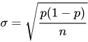
For example, suppose one randomly samples n people out of a large population and ask them whether they agree with a certain statement. The proportion of people who agree will of course depend on the sample. If groups of n people were sampled repeatedly and truly randomly, the proportions would follow an approximate normal distribution with mean equal to the true proportion p of agreement in the population and with standard deviation $\sigma ={\sqrt {\frac {p(1-p)}{n}}}$

Poisson approximation

The binomial distribution converges towards the Poisson distribution as the number of trials goes to infinity while the product np converges to a finite limit. Therefore, the Poisson distribution with parameter λ = np can be used as an approximation to B(n, p) of the binomial distribution if n is sufficiently large and p is sufficiently small. According to rules of thumb, this approximation is good if n ≥ 20 and p ≤ 0.05 such that np ≤ 1, or if n > 50 and p < 0.1 such that np < 5, or if n ≥ 100 and np ≤ 10.

Concerning the accuracy of Poisson approximation, see Novak, ch. 4, and references therein.

Limiting distributions

Poisson limit theorem: As n approaches ∞ and p approaches 0 with the product np held fixed, the Binomial(n, p) distribution approaches the Poisson distribution with expected value λ = np.
de Moivre-Laplace theorem: As n approaches ∞ while p remains fixed, the distribution of ${\frac {X-np}{\sqrt {np(1-p)}}}$ approaches the normal distribution with expected value 0 and variance 1. This result is sometimes loosely stated by saying that the distribution of X is asymptotically normal with expected value 0 and variance 1. This result is a specific case of the central limit theorem.

Beta distribution

The binomial distribution and beta distribution are different views of the same model of repeated Bernoulli trials. The binomial distribution is the PMF of k successes given n independent events each with a probability p of success. Mathematically, when α = k + 1 and β = n − k + 1, the beta distribution and the binomial distribution are related by a factor of n + 1: $\operatorname {Beta} (p;\alpha ;\beta )=(n+1)\mathrm {B} (k;n;p)$

Beta distributions also provide a family of prior probability distributions for binomial distributions in Bayesian inference: $P(p;\alpha ,\beta )={\frac {p^{\alpha -1}(1-p)^{\beta -1}}{\operatorname {Beta} (\alpha ,\beta )}}.$ Given a uniform prior, the posterior distribution for the probability of success p given n independent events with k observed successes is a beta distribution.

05Computational methods

Random number generation

Methods for random number generation where the marginal distribution is a binomial distribution are well-established. One way to generate random variates samples from a binomial distribution is to use an inversion algorithm. To do so, one must calculate the probability that Pr(X = k) for all values k from 0 through n. (These probabilities should sum to a value close to one, in order to encompass the entire sample space.) Then by using a pseudorandom number generator to generate samples uniformly between 0 and 1, one can transform the calculated samples into discrete numbers by using the probabilities calculated in the first step.

06History

This distribution was derived by Jacob Bernoulli. He considered the case where p = r/(r + s) where p is the probability of success and r and s are positive integers. Blaise Pascal had earlier considered the case where p = 1/2, tabulating the corresponding binomial coefficients in what is now recognized as Pascal's triangle.

Watch videos about Binomial distributionExplainers and documentaries on YouTube (opens in a new tab)

Sources and credits

This article is adapted from the Wikipedia article “Binomial distribution”, written by its contributors and licensed under CC BY-SA 4.0. Fathomly has changed the layout, removed citation markers, navigation and maintenance notices, and adjusted punctuation. This adapted version is shared under the same license. For references, see the original article.

Images, from Wikimedia Commons:

Binomial distribution pmf.svg by Tayste, Public domain
Pascal's triangle; binomial distribution.svg by Watchduck You can name the author as "T. Piesk", "Tilman Piesk" or "Watchduck"., Public domain
Binomial Distribution.svg by Cflm001 (talk), CC BY-SA 3.0

Fathomly is not affiliated with or endorsed by the Wikimedia Foundation. Spotted a problem? Tell us.

Binomial distribution

01Definitions

Probability mass function

Example

Cumulative distribution function

02Properties

Expected value and variance

Higher moments

Mode

Median

Tail bounds

03Statistical inference

Estimation of parameters

Confidence intervals for the parameter p

Wald method

Agresti-Coull method

Arcsine method

Wilson (score) method

Comparison

05Computational methods

Random number generation

06History

Sources and credits

Related topics

Logistic regression

Multinomial distribution

Negative binomial distribution