Encyclopedia

Axonometry

Process of projecting a 3D object onto a 2D plane

Wikipedia contributorsAdapted for Fathomly · View authors

7 min read
Source updated October 3, 2025

Axonometry is a graphical procedure belonging to descriptive geometry that generates a planar image of a three-dimensional object. The term "axonometry" means "to measure along axes", and indicates that the dimensions and scaling of the coordinate axes play a crucial role. The result of an axonometric procedure is a uniformly-scaled parallel projection of the object. In general, the resulting parallel projection is oblique (the rays are not perpendicular to the image plane); but in special cases the result is orthographic (the rays are perpendicular to the image plane), which in this context is called an orthogonal axonometry.

In technical drawing and in architecture, axonometric perspective is a form of two-dimensional representation of three-dimensional objects whose goal is to preserve the impression of volume or relief. Sometimes also called rapid perspective or artificial perspective, it differs from conical perspective and does not represent what the eye actually sees: in particular parallel lines remain parallel and distant objects are not reduced in size. It can be considered a conical perspective conique whose center has been pushed out to infinity, i.e. very far from the object observed.

The term axonometry is used both for the graphical procedure described below, as well as the image produced by this procedure.

Axonometry should not be confused with axonometric projection, which in English literature usually refers to orthogonal axonometry.

01Principle of axonometry

Pohlke's theorem is the basis for the following procedure to construct a scaled parallel projection of a three-dimensional object:

Select projections of the coordinate axes, such that all three coordinate axes are not collapsed to a single point or line. Usually the z-axis is vertical.
Select for these projections the foreshortenings, $v_{x}$ , $v_{y}$ and $v_{z}$ , where $v_{x},v_{y},v_{z}>0.$
The projection of a point is determined in three sub-steps (the result is independent of the order of these sub-steps):
- starting at the point ${\overline {O}}$ , move by the amount $v_{x}\cdot x$ in the direction of ${\overline {x}}$ , then
- move by the amount $v_{y}\cdot y$ in the direction of ${\overline {y}}$ , then
- move by the amount $v_{z}\cdot z$ in the direction of ${\overline {z}}$ and finally
Mark the final position as point ${\overline {P}}$ .

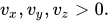
In order to obtain undistorted results, select the projections of the axes and foreshortenings carefully (see below). In order to produce an orthographic projection, only the projections of the coordinate axes are freely selected; the foreshortenings are fixed (see de:orthogonale Axonometrie).

The point is the projection of a point onto the projection plane Π. The foreshortenings are , and .

02The choice of the images of the axes and the foreshortenings

Notation:

$\alpha :$ angle between ${\overline {z}}$ -axis and ${\overline {x}}$ -axis
$\beta :$ angle between ${\overline {z}}$ -axis and ${\overline {y}}$ -axis
$\gamma :$ angle between ${\overline {x}}$ -axis and ${\overline {y}}$ -axis.

The angles can be chosen so that $0^{\circ }<\alpha +\beta <360^{\circ }\ .$
The foreshortenings: $0<\;v_{x},\;v_{y},\;v_{z}\ .$

Only for suitable choices of angles and foreshortenings does one get undistorted images. The next diagram shows the images of the unit cube for various angles and foreshortenings and gives some hints for how to make these personal choices.

In order to keep the drawing simple, one should choose simple foreshortenings, for example $1.0$ or $0.5$ .

If two foreshortenings are equal, the projection is called dimetric.
If the three foreshortenings are equal, the projection is called isometric.
If all foreshortenings are different, the projection is called trimetric.

The parameters in the diagram at right (e.g. of the house drawn on graph paper) are: $\alpha =135^{\circ },\beta =90^{\circ },\ v_{y}=v_{z}=1,\;v_{x}=1/{\sqrt {2}}\ .$ Hence it is a dimetric axonometry. The image plane is parallel to the y-z-plane and any planar figure parallel to the y-z-plane appears in its true shape.

Various axonometric images of a unit cube. (The image plane is parallel to the y-z-plane.) The left and the far right images look more like prolonged cuboids instead of a cube.

03Special axonometries

Commonly used projections and perspectives with angles between the transformed coordinate axes (α, β, γ), angles from the horizon (α_h, β_h, without γ_h = 90°) and scaling factors (*v_i*)
Name or property	α = ∠x̄z̄	β = ∠ȳz̄	γ = ∠x̄ȳ	α_h	β_h	v_x	v_y	v_z	v
Orthogonal, orthographic, planar	90°	0°	270°	0°	270°	v		0%	any
Trimetric	90° + α_h	90° + β_h	360° − α − β	any	any	any	any	any	any
Dimetric						any	v
Isometric						v
Normal						v			100%
Oblique, clinographic				< 90°	< 90°	any	any	any	tan(α_h)
Symmetric		α	360° − 2·α	< 90°	α_h				any
Equiangular	120°			30°					any
Normal, 1:1 isometric						v			100%
Standard, shortened isometric									${\textstyle {\sqrt {\frac {2}{3}}}$ ≈ 81%
Pixel, 1:2 isometric	116.6°		126.9°	arctan(v)					50%
Engineering	131.4°	97.2°	131.4°	arccos(⁠3/4⁠)	arcsin(⁠1/8⁠)	50%	v		100%
Cavalier	90° + α_h	90°	270° − α	any	0°	any
Cabinet, dimetric cavalier	90° + α_h		270° − α	any		< 100%
Standard, isometric cavalier	135°		135°	45°		v
Standard 1:2 cabinet	135°		135°	45°		50%	v
30° cabinet	116.6°		153.4°	arctan(v_x)
60° cabinet	153.4°		116.6°	arccot(v_x)
30° cavalier	120°		150°	30°		any
Aerial, bird's eye view	135°		90°	45°		v		any	100%
Military	135°			45°		v			100%
Planometric	90° + α_h	180° − α_h		any	90° − α_h				any
Normal planometric									100%
Shortened planometric									⁠2/3⁠ ≈ 67%

Engineer projection

In this case

the foreshortenings are: $v_{x}=0.5,\ v_{y}=v_{z}=1\$ (dimetric axonometry) and
the angles between the axes are: $\alpha =132^{\circ },\ \beta =97^{\circ }\ .$

These angles are marked on many German set squares.

Advantages of an engineer projection:

simple foreshortenings,
a uniformly scaled orthographic projection with scaling factor 1.06,
the contour of a sphere is a circle (in general, an ellipse) .

For more details: see de:Axonometrie.

Cavalier perspective, cabinet perspective

image plane parallel to y-z-plane.

In the literature the terms "cavalier perspective" and "cabinet perspective" are not uniformly defined. The above definition is the most general one. Often, further restrictions are applied. For example:

cabinet perspective: additionally choose $\alpha =135^{\circ }$ (oblique) and $v_{x}=0.5$ (dimetric),

cavalier perspective: additionally choose $\alpha =135^{\circ }$ (oblique) and $v_{x}=1$ (isometric).

Birds eye view, military projection

image plane parallel to x-y-plane.

military projection: additionally choose $v_{z}=1$ (isometric).

Such axonometries are often used for city maps, in order to keep horizontal figures undistorted.

Isometric axonometry

(Not to be confused with an isometry between metric spaces.)

For an isometric axonometry all foreshortenings are equal. The angles can be chosen arbitrarily, but a common choice is $\alpha =\beta =\gamma =120^{\circ }$ .

For the standard isometry or just isometry one chooses:

$v_{x}=v_{y}=v_{z}=1$ (all axes undistorted)
$\alpha =\beta =\gamma =120^{\circ }\ .$

The advantage of a standard isometry:

the coordinates can be taken unchanged,
the image is a scaled orthographic projection with scale factor ${\sqrt {1.5}}=1.225$ . Hence the image has a good impression and the contour of a sphere is a circle.
Some computer graphic systems (for example, xfig) provide a suitable raster (see diagram) as support.

In order to prevent scaling, one can choose the unhandy foreshortenings

$v_{x}=v_{y}=v_{z}={\sqrt {2/3}}$ (instead of 1)

and the image is an (unscaled) orthographic projection.

Axonometry (cavalier perspective) of a house on checked pattern paper.

04Circles in axonometry

A parallel projection of a circle is in general an ellipse. An important special case occurs, if the circle's plane is parallel to the image plane, the image of the circle is then a congruent circle. In the diagram, the circle contained in the front face is undistorted. If the image of a circle is an ellipse, one can map four points on orthogonal diameters and the surrounding square of tangents and in the image parallelogram fill-in an ellipse by hand. A better, but more time consuming method consists of drawing the images of two perpendicular diameters of the circle, which are conjugate diameters of the image ellipse, determining the axes of the ellipse with Rytz's construction and drawing the ellipse.

05Spheres in axonometry

In a general axonometry of a sphere the image contour is an ellipse. The contour of a sphere is a circle only in an orthogonal axonometry. But, as the engineer projection and the standard isometry are scaled orthographic projections, the contour of a sphere is a circle in these cases, as well. As the diagram shows, an ellipse as the contour of a sphere might be confusing, so, if a sphere is part of an object to be mapped, one should choose an orthogonal axonometry or an engineer projection or a standard isometry.

standard isometry: cube, cuboid, house and sphere

06Coordinate calculation

The Cartesian $x{\text{-}}y{\text{-}}z$ coordinate system with origin $O$ is still used in space. Let the drawing plane be equipped with a Cartesian $x'{\text{-}}y'$ coordinate system with origin ${\overline {O}}.$ An axonometry where ${\overline {O}}$ is the image point of $O$ can be represented by the map $f\colon \ \mathbb {R} ^{3}\to \mathbb {R} ^{2},$ $p={\begin{pmatrix}x\\y\\z\end{pmatrix}}\mapsto f(p)={\begin{pmatrix}x'\\y'\end{pmatrix}}$ which maps the coordinate vector $p\in \mathbb {R} ^{3}$ of a general point $P$ in space to the coordinate vector in $\mathbb {R} ^{2}$ of the image point ${\overline {P}}.$ The map $f$ is linear and can therefore be represented by its $2\!\times \!3$ transformation matrix $A\colon$ $f(p)=A\!\ p$ (matrix times vector). The three columns of $A$ are the image vectors $f(e_{x}),f(e_{y}),f(e_{z})\in \mathbb {R} ^{2}$ of the standard basis vectors $e_{x}={\begin{pmatrix}1\\0\\0\end{pmatrix}},\quad e_{y}={\begin{pmatrix}0\\1\\0\end{pmatrix}},\quad e_{z}={\begin{pmatrix}0\\0\\1\end{pmatrix}}$ and thus describe the ${\overline {x}},$ ${\overline {y}}$ und ${\overline {z}}$ image axes. They do not lie on a common straight line through the origin, i.e., the real $2\!\times \!3$ matrix $A$ has rank $2.$ Conversely, each such matrix generates an axonometry.

Examples

1. The factors $v_{x},v_{y},v_{z}$ and angles $\alpha ,\beta$ introduced above immediately lead to the transformation matrix $A={\begin{pmatrix}-v_{x}\sin \alpha &v_{y}\sin \beta &0\\v_{x}\cos \alpha &v_{y}\cos \beta &v_{z}\end{pmatrix}}.$ It is assumed that the $y'{\text{-}}$ axis and the ${\overline {z}}$ image axis point upwards and the $x'{\text{-}}$ axis points to the right.

2. In particular, $v_{x}=v_{y}=v_{z}=1$ and $\alpha =\beta =120^{\circ }$ give the standard isometry with the matrix $A={\begin{pmatrix}-{\frac {\sqrt {3}}{2}}&{\frac {\sqrt {3}}{2}}&0\\-{\frac {1}{2}}&-{\frac {1}{2}}&1\end{pmatrix}}.$ For instance, the vertex $p=(1,1,1)^{\mathsf {T}}$ of the unit cube is mapped to $f(p)=A\!\ p=(0,0)^{\mathsf {T}},$ as is the opposite vertex $(0,0,0)^{\mathsf {T}},$ where ${}^{\mathsf {T}}$ denotes transposition. As mentioned above, standard isometry is an orthographic projection scaled by the factor $\textstyle {\sqrt {3/2}}\,.$

3. Multiplying the last matrix by the reciprocal $\textstyle {\sqrt {2/3}}$ thus yields the transformation matrix $A={\begin{pmatrix}-{\frac {1}{\sqrt {2}}}&{\frac {1}{\sqrt {2}}}&0\\-{\frac {1}{\sqrt {6}}}&-{\frac {1}{\sqrt {6}}}&{\sqrt {\frac {2}{3}}}\end{pmatrix}}$ of an (unscaled) orthographic projection. Incidentally, in its transpose $A^{\mathsf {T}},$ both columns $e_{x}'={\begin{pmatrix}-{\frac {1}{\sqrt {2}}}\\{\frac {1}{\sqrt {2}}}\\[0.3ex]0\end{pmatrix}},\quad e_{y}'={\begin{pmatrix}-{\frac {1}{\sqrt {6}}}\\-{\frac {1}{\sqrt {6}}}\\{\sqrt {\frac {2}{3}}}\end{pmatrix}}$ are orthonormal, i.e., $e_{x}'\cdot e_{y}'=0$ and $e_{x}'\cdot e_{x}'=e_{y}'\cdot e_{y}'=1.$ This characterizes orthographic projections, as is shown exemplarily hereinafter.

4. Another orthographic projection is constructed, now conversely, starting with the orthonormal vectors $e_{x}'={\frac {1}{7}}{\begin{pmatrix}6\\-3\\-2\end{pmatrix}},\quad e_{y}'={\frac {1}{7}}{\begin{pmatrix}3\\2\\6\end{pmatrix}}.$ These two together with $e_{z}'=e_{x}'\times e_{y}'$ and $O$ define another Cartesian coordinate system in space. A general point $P$ in space now has another coordinate vector $p'=(x',y',z')^{\mathsf {T}}$ besides $p=(x,y,z)^{\mathsf {T}}.$ For these, always $E\!\ p'=p$ with the $3\!\times \!3$ change-of-basis matrix $E={\big (}e_{x}'\,{\big |}\,e_{y}'\,{\big |}\,e_{z}'{\big )}.$ As $E$ is orthogonal, $E^{-1}=E^{\mathsf {T}}$ and consequently $p'=E^{\mathsf {T}}p.$ The orthographic projection, which projects perpendicularly onto the $x'{\text{-}}y'{\text{-}}$ plane as the drawing plane, corresponds to omitting the bottom $z'{\text{-}}$ coordinate of $p'.$ Its transformation matrix is obtained accordingly from $E^{\mathsf {T}}$ by omitting the bottom row: $A={\frac {1}{7}}\,{\begin{pmatrix}6&-3&-2\\3&2&6\end{pmatrix}}.$ This can be used to calculate points in the adjacent drawing of the unit cube. For instance, the vertex $p=(1,1,1)^{\mathsf {T}}$ is mapped to $f(p)=A\!\ p={\big (}{\tfrac {1}{7}},{\tfrac {11}{7}}{\big )}{}^{\mathsf {T}}.$

various axonometries of a tower dimetric military projection: , dimetric engineering and cavalier projections: , isometric axonometry:

Watch videos about AxonometryExplainers and documentaries on YouTube (opens in a new tab)

Sources and credits

This article is adapted from the Wikipedia article “Axonometry”, written by its contributors and licensed under CC BY-SA 4.0. Fathomly has changed the layout, removed citation markers, navigation and maintenance notices, and adjusted punctuation. This adapted version is shared under the same license. For references, see the original article.

Images, from Wikimedia Commons:

Axonometrie-torbogen-c.svg by Ag2gaeh, CC BY-SA 4.0
Axonom-def.svg by Ag2gaeh, CC BY-SA 4.0
Axo-parameter-gen.svg by Ag2gaeh, CC BY-SA 4.0
Axonometry-var14.svg by Ag2gaeh, CC BY-SA 4.0
Haus-karo-axonometrie.svg by Ag2gaeh, CC BY-SA 4.0
Axo-parameter-spec.svg by Ag2gaeh, CC BY-SA 4.0
Axo-iso-beisp.svg by Ag2gaeh, CC BY-SA 4.0
Axo-examples.svg by Ag2gaeh, CC BY-SA 4.0

Fathomly is not affiliated with or endorsed by the Wikimedia Foundation. Spotted a problem? Tell us.