Encyclopedia

AdaBoost

Adaptive boosting based classification algorithm

Wikipedia contributorsAdapted for Fathomly · View authors

9 min read
Source updated September 7, 2026

AdaBoost (short for Adaptive Boosting) is a statistical classification meta-algorithm formulated by Yoav Freund and Robert Schapire in 1995, who won the 2003 Gödel Prize for their work. It can be used in conjunction with many types of learning algorithm to improve performance. The output of multiple weak learners is combined into a weighted sum that represents the final output of the boosted classifier. Usually, AdaBoost is presented for binary classification, although it can be generalized to multiple classes or bounded intervals of real values.

AdaBoost is adaptive in the sense that subsequent weak learners (models) are adjusted in favor of instances misclassified by previous models. In some problems, it can be less susceptible to overfitting than other learning algorithms. The individual learners can be weak, but as long as the performance of each one is slightly better than random guessing, the final model can be proven to converge to a strong learner.

Although AdaBoost is typically used to combine weak base learners (such as decision stumps), it has been shown to also effectively combine strong base learners (such as deeper decision trees), producing an even more accurate model.

Every learning algorithm tends to suit some problem types better than others, and typically has many different parameters and configurations to adjust before it achieves optimal performance on a dataset. AdaBoost (with decision trees as the weak learners) is often referred to as the best out-of-the-box classifier. When used with decision tree learning, information gathered at each stage of the AdaBoost algorithm about the relative 'hardness' of each training sample is fed into the tree-growing algorithm such that later trees tend to focus on harder-to-classify examples.

01Training

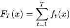
AdaBoost refers to a particular method of training a boosted classifier. A boosted classifier is a classifier of the form $F_{T}(x)=\sum _{t=1}^{T}f_{t}(x)$ where each $f_{t}$ is a weak learner that takes an object $x$ as input and returns a value indicating the class of the object. For example, in the two-class problem, the sign of the weak learner's output identifies the predicted object class and the absolute value gives the confidence in that classification.

Each weak learner produces an output hypothesis $h$ which fixes a prediction $h(x_{i})$ for each sample in the training set. At each iteration $t$ , a weak learner is selected and assigned a coefficient $\alpha _{t}$ such that the total training error $E_{t}$ of the resulting $t$ -stage boosted classifier is minimized.

$E_{t}=\sum _{i}E[F_{t-1}(x_{i})+\alpha _{t}h(x_{i})]$

Here $F_{t-1}(x)$ is the boosted classifier that has been built up to the previous stage of training and $f_{t}(x)=\alpha _{t}h(x)$ is the weak learner that is being considered for addition to the final classifier.

Weighting

At each iteration of the training process, a weight $w_{i,t}$ is assigned to each sample in the training set equal to the current error $E(F_{t-1}(x_{i}))$ on that sample. These weights can be used in the training of the weak learner. For instance, decision trees can be grown which favor the splitting of sets of samples with large weights.

02Derivation

This derivation follows Rojas (2009):

Suppose we have a data set $\{(x_{1},y_{1}),\ldots ,(x_{N},y_{N})\}$ where each item $x_{i}$ has an associated class $y_{i}\in \{-1,1\}$ , and a set of weak classifiers $\{k_{1},\ldots ,k_{L}\}$ each of which outputs a classification $k_{j}(x_{i})\in \{-1,1\}$ for each item. After the $(m-1)$ -th iteration our boosted classifier is a linear combination of the weak classifiers of the form: $C_{(m-1)}(x_{i})=\alpha _{1}k_{1}(x_{i})+\cdots +\alpha _{m-1}k_{m-1}(x_{i}),$ where the class will be the sign of $C_{(m-1)}(x_{i})$ . At the $m$ -th iteration we want to extend this to a better boosted classifier by adding another weak classifier $k_{m}$ , with another weight $\alpha _{m}$ : $C_{m}(x_{i})=C_{(m-1)}(x_{i})+\alpha _{m}k_{m}(x_{i})$

So it remains to determine which weak classifier is the best choice for $k_{m}$ , and what its weight $\alpha _{m}$ should be. We define the total error $E$ of $C_{m}$ as the sum of its exponential loss on each data point, given as follows: $E=\sum _{i=1}^{N}e^{-y_{i}C_{m}(x_{i})}=\sum _{i=1}^{N}e^{-y_{i}C_{(m-1)}(x_{i})}e^{-y_{i}\alpha _{m}k_{m}(x_{i})}$

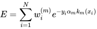
Letting $w_{i}^{(1)}=1$ and $w_{i}^{(m)}=e^{-y_{i}C_{m-1}(x_{i})}$ for $m>1$ , we have: $E=\sum _{i=1}^{N}w_{i}^{(m)}e^{-y_{i}\alpha _{m}k_{m}(x_{i})}$

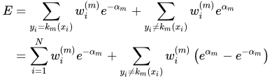
We can split this summation between those data points that are correctly classified by $k_{m}$ (so $y_{i}k_{m}(x_{i})=1$ ) and those that are misclassified (so $y_{i}k_{m}(x_{i})=-1$ ): ${\begin{aligned}E&=\sum _{y_{i}=k_{m}(x_{i})}w_{i}^{(m)}e^{-\alpha _{m}}+\sum _{y_{i}\neq k_{m}(x_{i})}w_{i}^{(m)}e^{\alpha _{m}}\\&=\sum _{i=1}^{N}w_{i}^{(m)}e^{-\alpha _{m}}+\sum _{y_{i}\neq k_{m}(x_{i})}w_{i}^{(m)}\left(e^{\alpha _{m}}-e^{-\alpha _{m}}\right)\end{aligned}}$

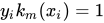
Since the only part of the right-hand side of this equation that depends on $k_{m}$ is ${\textstyle \sum _{y_{i}\neq k_{m}(x_{i})}w_{i}^{(m)}$ , we see that the $k_{m}$ that minimizes $E$ is the one in the set $\{k_{1},\ldots ,k_{L}\}$ that minimizes ${\textstyle \sum _{y_{i}\neq k_{m}(x_{i})}w_{i}^{(m)}$ [assuming that $\alpha _{m}>0$ ], i.e. the weak classifier with the lowest weighted error (with weights $w_{i}^{(m)}=e^{-y_{i}C_{m-1}(x_{i})}$ ).

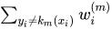
To determine the desired weight $\alpha _{m}$ that minimizes $E$ with the $k_{m}$ that we just determined, we differentiate: ${\frac {dE}{d\alpha _{m}}}={\frac {d(\sum _{y_{i}=k_{m}(x_{i})}w_{i}^{(m)}e^{-\alpha _{m}}+\sum _{y_{i}\neq k_{m}(x_{i})}w_{i}^{(m)}e^{\alpha _{m}})}{d\alpha _{m}}}$

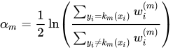
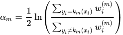
The value of $\alpha _{m}$ that minimizes the above expression is: $\alpha _{m}={\frac {1}{2}}\ln \left({\frac {\sum _{y_{i}=k_{m}(x_{i})}w_{i}^{(m)}}{\sum _{y_{i}\neq k_{m}(x_{i})}w_{i}^{(m)}}}\right)$

Proof

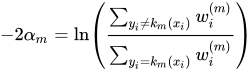
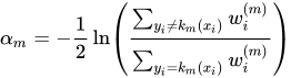
${\frac {dE}{d\alpha _{m}}}=-\sum _{y_{i}=k_{m}(x_{i})}w_{i}^{(m)}e^{-\alpha _{m}}+\sum _{y_{i}\neq k_{m}(x_{i})}w_{i}^{(m)}e^{\alpha _{m}}=0$ because $e^{-\alpha _{m}}$ does not depend on $i$ $e^{-\alpha _{m}}\sum _{y_{i}=k_{m}(x_{i})}w_{i}^{(m)}=e^{\alpha _{m}}\sum _{y_{i}\neq k_{m}(x_{i})}w_{i}^{(m)}$ $-\alpha _{m}+\ln \left(\sum _{y_{i}=k_{m}(x_{i})}w_{i}^{(m)}\right)=\alpha _{m}+\ln \left(\sum _{y_{i}\neq k_{m}(x_{i})}w_{i}^{(m)}\right)$ $-2\alpha _{m}=\ln \left({\dfrac {\sum _{y_{i}\neq k_{m}(x_{i})}w_{i}^{(m)}}{\sum _{y_{i}=k_{m}(x_{i})}w_{i}^{(m)}}}\right)$ $\alpha _{m}=-{\dfrac {1}{2}}\ln \left({\dfrac {\sum _{y_{i}\neq k_{m}(x_{i})}w_{i}^{(m)}}{\sum _{y_{i}=k_{m}(x_{i})}w_{i}^{(m)}}}\right)$ $\alpha _{m}={\dfrac {1}{2}}\ln \left({\dfrac {\sum _{y_{i}=k_{m}(x_{i})}w_{i}^{(m)}}{\sum _{y_{i}\neq k_{m}(x_{i})}w_{i}^{(m)}}}\right)$

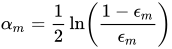
We calculate the weighted error rate of the weak classifier to be $\epsilon _{m}={\frac {\sum _{y_{i}\neq k_{m}(x_{i})}w_{i}^{(m)}}{\sum _{i=1}^{N}w_{i}^{(m)}}}$ , so it follows that: $\alpha _{m}={\frac {1}{2}}\ln \left({\frac {1-\epsilon _{m}}{\epsilon _{m}}}\right)$ which is the negative logit function multiplied by 0.5. Due to the convexity of $E$ as a function of $\alpha _{m}$ , this new expression for $\alpha _{m}$ gives the global minimum of the loss function.

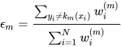
Note: This derivation only applies when $k_{m}(x_{i})\in \{-1,1\}$ , though it can be a good starting guess in other cases, such as when the weak learner is biased ( $k_{m}(x)\in \{a,b\},a\neq -b$ ), has multiple leaves ( $k_{m}(x)\in \{a,b,\dots ,n\}$ ) or is some other function $k_{m}(x)\in \mathbb {R}$ .

Thus we have derived the AdaBoost algorithm: At each iteration, choose the classifier $k_{m}$ , which minimizes the total weighted error ${\textstyle \sum _{y_{i}\neq k_{m}(x_{i})}w_{i}^{(m)}$ , use this to calculate the error rate $\epsilon _{m}={\frac {\sum _{y_{i}\neq k_{m}(x_{i})}w_{i}^{(m)}}{\sum _{i=1}^{N}w_{i}^{(m)}}}$ , use this to calculate the weight $\alpha _{m}={\frac {1}{2}}\ln \left({\frac {1-\epsilon _{m}}{\epsilon _{m}}}\right)$ , and finally use this to improve the boosted classifier $C_{m-1}$ to $C_{m}=C_{(m-1)}+\alpha _{m}k_{m}$ .

03Statistical understanding of boosting

Boosting is a form of linear regression in which the features of each sample $x_{i}$ are the outputs of some weak learner $h$ applied to $x_{i}$ .

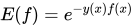
While regression tries to fit $F(x)$ to $y(x)$ as precisely as possible without loss of generalization, typically using least square error $E(f)=(y(x)-f(x))^{2}$ , whereas the AdaBoost error function $E(f)=e^{-y(x)f(x)}$ takes into account the fact that only the sign of the final result is used, thus $|F(x)|$ can be far larger than 1 without increasing error. However, the exponential increase in the error for sample $x_{i}$ as $-y(x_{i})f(x_{i})$ increases, resulting in excessive weights being assigned to outliers.

One feature of the choice of exponential error function is that the error of the final additive model is the product of the error of each stage, that is, $e^{\sum _{m}-y_{i}f_{m}(x_{i})}=\prod _{m}e^{-y_{i}f_{m}(x_{i})}$ . Thus it can be seen that the weight update in the AdaBoost algorithm is equivalent to recalculating the error on $F_{t}(x)$ after each stage.

There is a lot of flexibility allowed in the choice of loss function. As long as the loss function is monotonic and continuously differentiable, the classifier is always driven toward purer solutions. Zhang (2004) provides a loss function based on least squares, a modified Huber loss function: $\phi (y,f(x))={\begin{cases}-4yf(x)&{\text{if }}yf(x)<-1,\\(yf(x)-1)^{2}&{\text{if }}-1\leq yf(x)\leq 1.\\0&{\text{if }}yf(x)>1\end{cases}}$

This function is more well-behaved than LogitBoost for $f(x)$ close to 1 or -1, does not penalise ‘overconfident’ predictions ( $yf(x)>1$ ), unlike unmodified least squares, and only penalises samples misclassified with confidence greater than 1 linearly, as opposed to quadratically or exponentially, and is thus less susceptible to the effects of outliers.

04Boosting as gradient descent

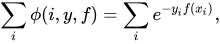
Boosting can be seen as minimization of a convex loss function over a convex set of functions. Specifically, the loss being minimized by AdaBoost is the exponential loss $\sum _{i}\phi (i,y,f)=\sum _{i}e^{-y_{i}f(x_{i})},$ whereas LogitBoost performs logistic regression, minimizing $\sum _{i}\phi (i,y,f)=\sum _{i}\ln \left(1+e^{-y_{i}f(x_{i})}\right).$

In the gradient descent analogy, the output of the classifier for each training point is considered a point $\left(F_{t}(x_{1}),\dots ,F_{t}(x_{n})\right)$ in n-dimensional space, where each axis corresponds to a training sample, each weak learner $h(x)$ corresponds to a vector of fixed orientation and length, and the goal is to reach the target point $(y_{1},\dots ,y_{n})$ (or any region where the value of loss function $E_{T}(x_{1},\dots ,x_{n})$ is less than the value at that point), in the fewest steps. Thus AdaBoost algorithms perform either Cauchy (find $h(x)$ with the steepest gradient, choose $\alpha$ to minimize test error) or Newton (choose some target point, find $\alpha h(x)$ that brings $F_{t}$ closest to that point) optimization of training error.

05Example algorithm (Discrete AdaBoost)

With:

Samples $x_{1}\dots x_{n}$
Desired outputs $y_{1}\dots y_{n},y\in \{-1,1\}$
Initial weights $w_{1,1}\dots w_{n,1}$ set to ${\frac {1}{n}}$
Error function $E(f(x),y_{i})=e^{-y_{i}f(x_{i})}$
Weak learners $h\colon x\rightarrow \{-1,1\}$

For $t$ in $1\dots T$ :

Choose :
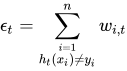
- Find weak learner $h_{t}(x)$ that minimizes $\epsilon _{t}$ , the weighted sum error for misclassified points $\epsilon _{t}=\sum _{\stackrel {i=1}{h_{t}(x_{i})\neq y_{i}}}^{n}w_{i,t}$
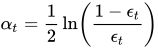
- Choose $\alpha _{t}={\frac {1}{2}}\ln \left({\frac {1-\epsilon _{t}}{\epsilon _{t}}}\right)$
Add to ensemble:
- $F_{t}(x)=F_{t-1}(x)+\alpha _{t}h_{t}(x)$
Update weights:
- $w_{i,t+1}=w_{i,t}e^{-y_{i}\alpha _{t}h_{t}(x_{i})}$ for $i$ in $1\dots n$
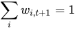
- Renormalize $w_{i,t+1}$ such that $\sum _{i}w_{i,t+1}=1$
- (Note: It can be shown that ${\frac {\sum _{h_{t}(x_{i})=y_{i}}w_{i,t+1}}{\sum _{h_{t}(x_{i})\neq y_{i}}w_{i,t+1}}}={\frac {\sum _{h_{t}(x_{i})=y_{i}}w_{i,t}}{\sum _{h_{t}(x_{i})\neq y_{i}}w_{i,t}}}$ at every step, which can simplify the calculation of the new weights.)

06Variants

Real AdaBoost

The output of decision trees is a class probability estimate $p(x)=P(y=1|x)$ , the probability that $x$ is in the positive class. Friedman, Hastie and Tibshirani derive an analytical minimizer for $e^{-y\left(F_{t-1}(x)+f_{t}(p(x))\right)}$ for some fixed $p(x)$ (typically chosen using weighted least squares error):

$f_{t}(x)={\frac {1}{2}}\ln \left({\frac {x}{1-x}}\right)$ .

Thus, rather than multiplying the output of the entire tree by some fixed value, each leaf node is changed to output half the logit transform of its previous value.

LogitBoost

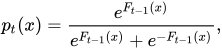
LogitBoost represents an application of established logistic regression techniques to the AdaBoost method. Rather than minimizing error with respect to y, weak learners are chosen to minimize the (weighted least-squares) error of $f_{t}(x)$ with respect to $z_{t}={\frac {y^{*}-p_{t}(x)}{2p_{t}(x)(1-p_{t}(x))}},$ where $p_{t}(x)={\frac {e^{F_{t-1}(x)}}{e^{F_{t-1}(x)}+e^{-F_{t-1}(x)}}},$ $w_{t}=p_{t}(x)(1-p_{t}(x))$ $y^{*}={\frac {y+1}{2}}.$

That is $z_{t}$ is the Newton-Raphson approximation of the minimizer of the log-likelihood error at stage $t$ , and the weak learner $f_{t}$ is chosen as the learner that best approximates $z_{t}$ by weighted least squares.

As p approaches either 1 or 0, the value of $p_{t}(x_{i})(1-p_{t}(x_{i}))$ becomes very small and the z term, which is large for misclassified samples, can become numerically unstable, due to machine precision rounding errors. This can be overcome by enforcing some limit on the absolute value of z and the minimum value of w

Gentle AdaBoost

While previous boosting algorithms choose $f_{t}$ greedily, minimizing the overall test error as much as possible at each step, GentleBoost features a bounded step size. $f_{t}$ is chosen to minimize ${\textstyle \sum _{i}w_{t,i}(y_{i}-f_{t}(x_{i}))^{2}$ , and no further coefficient is applied. Thus, in the case where a weak learner exhibits perfect classification performance, GentleBoost chooses $f_{t}(x)=\alpha _{t}h_{t}(x)$ exactly equal to $y$ , while steepest descent algorithms try to set $\alpha _{t}=\infty$ . Empirical observations about the good performance of GentleBoost appear to back up Schapire and Singer's remark that allowing excessively large values of $\alpha$ can lead to poor generalization performance.

Early termination

A technique for speeding up processing of boosted classifiers, early termination refers to only testing each potential object with as many layers of the final classifier necessary to meet some confidence threshold, speeding up computation for cases where the class of the object can easily be determined. One such scheme is the object detection framework introduced by Viola and Jones: in an application with significantly more negative samples than positive, a cascade of separate boost classifiers is trained, the output of each stage biased such that some acceptably small fraction of positive samples is mislabeled as negative, and all samples marked as negative after each stage are discarded. If 50% of negative samples are filtered out by each stage, only a very small number of objects would pass through the entire classifier, reducing computation effort. This method has since been generalized, with a formula provided for choosing optimal thresholds at each stage to achieve some desired false positive and false negative rate.

In the field of statistics, where AdaBoost is more commonly applied to problems of moderate dimensionality, early stopping is used as a strategy to reduce overfitting. A validation set of samples is separated from the training set, performance of the classifier on the samples used for training is compared to performance on the validation samples, and training is terminated if performance on the validation sample is seen to decrease even as performance on the training set continues to improve.

Totally corrective algorithms

For steepest descent versions of AdaBoost, where $\alpha _{t}$ is chosen at each layer t to minimize test error, the next layer added is said to be maximally independent of layer t: it is unlikely to choose a weak learner t+1 that is similar to learner t. However, there remains the possibility that t+1 produces similar information to some other earlier layer. Totally corrective algorithms, such as LPBoost, optimize the value of every coefficient after each step, such that new layers added are always maximally independent of every previous layer. This can be accomplished by backfitting, linear programming or some other method.

Pruning

Pruning is the process of removing poorly performing weak classifiers to improve memory and execution-time cost of the boosted classifier. The simplest methods, which can be particularly effective in conjunction with totally corrective training, are weight- or margin-trimming: when the coefficient, or the contribution to the total test error, of some weak classifier falls below a certain threshold, that classifier is dropped. Margineantu & Dietterich suggested an alternative criterion for trimming: weak classifiers should be selected such that the diversity of the ensemble is maximized. If two weak learners produce very similar outputs, efficiency can be improved by removing one of them and increasing the coefficient of the remaining weak learner.

Watch videos about AdaBoostExplainers and documentaries on YouTube (opens in a new tab)

Sources and credits

This article is adapted from the Wikipedia article “AdaBoost”, written by its contributors and licensed under CC BY-SA 4.0. Fathomly has changed the layout, removed citation markers, navigation and maintenance notices, and adjusted punctuation. This adapted version is shared under the same license. For references, see the original article.

Fathomly is not affiliated with or endorsed by the Wikimedia Foundation. Spotted a problem? Tell us.