Encyclopedia

Standard normal table

Table of probabilities related to the normal distribution

Wikipedia contributorsAdapted for Fathomly · View authors

10 min read
Source updated May 10, 2026

In statistics, a standard normal table, also called the unit normal table or Z table, is a mathematical table for the values of Φ, the cumulative distribution function of the normal distribution. It is used to find the probability that a statistic is observed below, above, or between values on the standard normal distribution, and by extension, any normal distribution. Since probability tables cannot be printed for every normal distribution, as there are an infinite variety of normal distributions, it is common practice to convert a normal to a standard normal (known as a z-score) and then use the standard normal table to find probabilities.

01Normal and standard normal distribution

Normal distributions are symmetrical, bell-shaped distributions that are useful in describing real-world data. The standard normal distribution, represented by Z, is the normal distribution having a mean of 0 and a standard deviation of 1.

Conversion

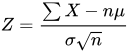
If X is a random variable from a normal distribution with mean μ and standard deviation σ, its Z-score may be calculated from X by subtracting μ and dividing by the standard deviation:

$Z={\frac {X-\mu }{\sigma }}$

If ${\overline {X}}$ is the mean of a sample of size n from some population in which the mean is μ and the standard deviation is σ, the standard error is ⁠ ${\tfrac {\sigma }{\sqrt {n}}}:$ ⁠

$Z={\frac {{\overline {X}}-\mu }{\sigma /{\sqrt {n}}}}$

If ${\textstyle \sum X$ is the total of a sample of size n from some population in which the mean is μ and the standard deviation is σ, the expected total is nμ and the standard error is ⁠ $\sigma {\sqrt {n}}:$ ⁠

$Z={\frac {\sum {X}-n\mu }{\sigma {\sqrt {n}}}}$

02Reading a Z table

Formatting / layout

Z tables are typically composed as follows:

The label for rows contains the integer part and the first decimal place of Z.
The label for columns contains the second decimal place of Z.
The values within the table are the probabilities corresponding to the table type. These probabilities are calculations of the area under the normal curve from the starting point (0 for cumulative from mean, negative infinity for cumulative and positive infinity for complementary cumulative) to Z.

Example: To find 0.69, one would look down the rows to find 0.6 and then across the columns to 0.09 which would yield a probability of 0.25490 for a cumulative from mean table or 0.75490 from a cumulative table.

To find a negative value such as , 0.83, one could use a cumulative table for negative z-values which yield a probability of 0.20327.

But since the normal distribution curve is symmetrical, probabilities for only positive values of Z are typically given. The user might have to use a complementary operation on the absolute value of Z, as in the example below.

Types of tables

Z tables use at least three different conventions:

Cumulative from mean: gives a probability that a statistic is between 0 (mean) and Z. Example: Prob(0 ≤ Z ≤ 0.69) = 0.2549.
Cumulative: gives a probability that a statistic is less than Z. This equates to the area of the distribution below Z. Example: Prob(Z ≤ 0.69) = 0.7549.
Complementary cumulative: gives a probability that a statistic is greater than Z. This equates to the area of the distribution above Z.; Example: Find Prob(Z ≥ 0.69). Since this is the portion of the area above Z, the proportion that is greater than Z is found by subtracting Z from 1. That is Prob(Z ≥ 0.69) = 1 − Prob(Z ≤ 0.69) or Prob(Z ≥ 0.69) = 1 − 0.7549 = 0.2451.

03Table examples

Cumulative from minus infinity to Z

This table gives a probability that a statistic is between minus infinity and Z.

$f(z)=\Phi (z)$

The values are calculated using the cumulative distribution function of a standard normal distribution with mean of zero and standard deviation of one, usually denoted with the capital Greek letter $\Phi$ (phi), is the integral

$\Phi (z)={\frac {1}{\sqrt {2\pi }}}\int _{-\infty }^{z}e^{-t^{2}/2}\,dt$

$\Phi$ (z) is related to the error function, or erf(z).

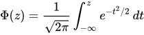
$\Phi (z)={\frac {1}{2}}\left[1+\operatorname {erf} \left({\frac {z}{\sqrt {2}}}\right)\right]$

Note that for z = 1, 2, 3, one obtains (after multiplying by 2 to account for the [−z,z] interval) the results f (z) = 0.6827, 0.9545, 0.9974, characteristic of the 68-95-99.7 rule.

Cumulative (less than Z)

This table gives a probability that a statistic is less than Z (i.e. between negative infinity and Z).

z	−0.00	−0.01	−0.02	−0.03	−0.04	−0.05	−0.06	−0.07	−0.08	−0.09
-3.9	0.00005	0.00005	0.00004	0.00004	0.00004	0.00004	0.00004	0.00004	0.00003	0.00003
-3.8	0.00007	0.00007	0.00007	0.00006	0.00006	0.00006	0.00006	0.00005	0.00005	0.00005
-3.7	0.00011	0.00010	0.00010	0.00010	0.00009	0.00009	0.00008	0.00008	0.00008	0.00008
-3.6	0.00016	0.00015	0.00015	0.00014	0.00014	0.00013	0.00013	0.00012	0.00012	0.00011
-3.5	0.00023	0.00022	0.00022	0.00021	0.00020	0.00019	0.00019	0.00018	0.00017	0.00017
-3.4	0.00034	0.00032	0.00031	0.00030	0.00029	0.00028	0.00027	0.00026	0.00025	0.00024
-3.3	0.00048	0.00047	0.00045	0.00043	0.00042	0.00040	0.00039	0.00038	0.00036	0.00035
-3.2	0.00069	0.00066	0.00064	0.00062	0.00060	0.00058	0.00056	0.00054	0.00052	0.00050
-3.1	0.00097	0.00094	0.00090	0.00087	0.00084	0.00082	0.00079	0.00076	0.00074	0.00071
-3.0	0.00135	0.00131	0.00126	0.00122	0.00118	0.00114	0.00111	0.00107	0.00104	0.00100
-2.9	0.00187	0.00181	0.00175	0.00169	0.00164	0.00159	0.00154	0.00149	0.00144	0.00139
-2.8	0.00256	0.00248	0.00240	0.00233	0.00226	0.00219	0.00212	0.00205	0.00199	0.00193
-2.7	0.00347	0.00336	0.00326	0.00317	0.00307	0.00298	0.00289	0.00280	0.00272	0.00264
-2.6	0.00466	0.00453	0.00440	0.00427	0.00415	0.00402	0.00391	0.00379	0.00368	0.00357
-2.5	0.00621	0.00604	0.00587	0.00570	0.00554	0.00539	0.00523	0.00508	0.00494	0.00480
-2.4	0.00820	0.00798	0.00776	0.00755	0.00734	0.00714	0.00695	0.00676	0.00657	0.00639
-2.3	0.01072	0.01044	0.01017	0.00990	0.00964	0.00939	0.00914	0.00889	0.00866	0.00842
-2.2	0.01390	0.01355	0.01321	0.01287	0.01255	0.01222	0.01191	0.01160	0.01130	0.01101
-2.1	0.01786	0.01743	0.01700	0.01659	0.01618	0.01578	0.01539	0.01500	0.01463	0.01426
-2.0	0.02275	0.02222	0.02169	0.02118	0.02068	0.02018	0.01970	0.01923	0.01876	0.01831
−1.9	0.02872	0.02807	0.02743	0.02680	0.02619	0.02559	0.02500	0.02442	0.02385	0.02330
−1.8	0.03593	0.03515	0.03438	0.03362	0.03288	0.03216	0.03144	0.03074	0.03005	0.02938
−1.7	0.04457	0.04363	0.04272	0.04182	0.04093	0.04006	0.03920	0.03836	0.03754	0.03673
−1.6	0.05480	0.05370	0.05262	0.05155	0.05050	0.04947	0.04846	0.04746	0.04648	0.04551
−1.5	0.06681	0.06552	0.06426	0.06301	0.06178	0.06057	0.05938	0.05821	0.05705	0.05592

−1.4	0.08076	0.07927	0.07780	0.07636	0.07493	0.07353	0.07215	0.07078	0.06944	0.06811
−1.3	0.09680	0.09510	0.09342	0.09176	0.09012	0.08851	0.08692	0.08534	0.08379	0.08226
−1.2	0.11507	0.11314	0.11123	0.10935	0.10749	0.10565	0.10383	0.10204	0.10027	0.09853
−1.1	0.13567	0.13350	0.13136	0.12924	0.12714	0.12507	0.12302	0.12100	0.11900	0.11702
−1.0	0.15866	0.15625	0.15386	0.15151	0.14917	0.14686	0.14457	0.14231	0.14007	0.13786

−0.9	0.18406	0.18141	0.17879	0.17619	0.17361	0.17106	0.16853	0.16602	0.16354	0.16109
−0.8	0.21186	0.20897	0.20611	0.20327	0.20045	0.19766	0.19489	0.19215	0.18943	0.18673
−0.7	0.24196	0.23885	0.23576	0.23270	0.22965	0.22663	0.22363	0.22065	0.21770	0.21476
−0.6	0.27425	0.27093	0.26763	0.26435	0.26109	0.25785	0.25463	0.25143	0.24825	0.24510
−0.5	0.30854	0.30503	0.30153	0.29806	0.29460	0.29116	0.28774	0.28434	0.28096	0.27760

−0.4	0.34458	0.34090	0.33724	0.33360	0.32997	0.32636	0.32276	0.31918	0.31561	0.31207
−0.3	0.38209	0.37828	0.37448	0.37070	0.36693	0.36317	0.35942	0.35569	0.35197	0.34827
−0.2	0.42074	0.41683	0.41294	0.40905	0.40517	0.40129	0.39743	0.39358	0.38974	0.38591
−0.1	0.46017	0.45620	0.45224	0.44828	0.44433	0.44038	0.43644	0.43251	0.42858	0.42465
−0.0	0.50000	0.49601	0.49202	0.48803	0.48405	0.48006	0.47608	0.47210	0.46812	0.46414
z	−0.00	−0.01	−0.02	−0.03	−0.04	−0.05	−0.06	−0.07	−0.08	−0.09

z	+ 0.00	+ 0.01	+ 0.02	+ 0.03	+ 0.04	+ 0.05	+ 0.06	+ 0.07	+ 0.08	+ 0.09
0.0	0.50000	0.50399	0.50798	0.51197	0.51595	0.51994	0.52392	0.52790	0.53188	0.53586
0.1	0.53983	0.54380	0.54776	0.55172	0.55567	0.55962	0.56360	0.56749	0.57142	0.57535
0.2	0.57926	0.58317	0.58706	0.59095	0.59483	0.59871	0.60257	0.60642	0.61026	0.61409
0.3	0.61791	0.62172	0.62552	0.62930	0.63307	0.63683	0.64058	0.64431	0.64803	0.65173
0.4	0.65542	0.65910	0.66276	0.66640	0.67003	0.67364	0.67724	0.68082	0.68439	0.68793

0.5	0.69146	0.69497	0.69847	0.70194	0.70540	0.70884	0.71226	0.71566	0.71904	0.72240
0.6	0.72575	0.72907	0.73237	0.73565	0.73891	0.74215	0.74537	0.74857	0.75175	0.75490
0.7	0.75804	0.76115	0.76424	0.76730	0.77035	0.77337	0.77637	0.77935	0.78230	0.78524
0.8	0.78814	0.79103	0.79389	0.79673	0.79955	0.80234	0.80511	0.80785	0.81057	0.81327
0.9	0.81594	0.81859	0.82121	0.82381	0.82639	0.82894	0.83147	0.83398	0.83646	0.83891

1.0	0.84134	0.84375	0.84614	0.84849	0.85083	0.85314	0.85543	0.85769	0.85993	0.86214
1.1	0.86433	0.86650	0.86864	0.87076	0.87286	0.87493	0.87698	0.87900	0.88100	0.88298
1.2	0.88493	0.88686	0.88877	0.89065	0.89251	0.89435	0.89617	0.89796	0.89973	0.90147
1.3	0.90320	0.90490	0.90658	0.90824	0.90988	0.91149	0.91308	0.91466	0.91621	0.91774
1.4	0.91924	0.92073	0.92220	0.92364	0.92507	0.92647	0.92785	0.92922	0.93056	0.93189

1.5	0.93319	0.93448	0.93574	0.93699	0.93822	0.93943	0.94062	0.94179	0.94295	0.94408
1.6	0.94520	0.94630	0.94738	0.94845	0.94950	0.95053	0.95154	0.95254	0.95352	0.95449
1.7	0.95543	0.95637	0.95728	0.95818	0.95907	0.95994	0.96080	0.96164	0.96246	0.96327
1.8	0.96407	0.96485	0.96562	0.96638	0.96712	0.96784	0.96856	0.96926	0.96995	0.97062
1.9	0.97128	0.97193	0.97257	0.97320	0.97381	0.97441	0.97500	0.97558	0.97615	0.97670

2.0	0.97725	0.97778	0.97831	0.97882	0.97932	0.97982	0.98030	0.98077	0.98124	0.98169
2.1	0.98214	0.98257	0.98300	0.98341	0.98382	0.98422	0.98461	0.98500	0.98537	0.98574
2.2	0.98610	0.98645	0.98679	0.98713	0.98745	0.98778	0.98809	0.98840	0.98870	0.98899
2.3	0.98928	0.98956	0.98983	0.99010	0.99036	0.99061	0.99086	0.99111	0.99134	0.99158
2.4	0.99180	0.99202	0.99224	0.99245	0.99266	0.99286	0.99305	0.99324	0.99343	0.99361

2.5	0.99379	0.99396	0.99413	0.99430	0.99446	0.99461	0.99477	0.99492	0.99506	0.99520
2.6	0.99534	0.99547	0.99560	0.99573	0.99585	0.99598	0.99609	0.99621	0.99632	0.99643
2.7	0.99653	0.99664	0.99674	0.99683	0.99693	0.99702	0.99711	0.99720	0.99728	0.99736
2.8	0.99744	0.99752	0.99760	0.99767	0.99774	0.99781	0.99788	0.99795	0.99801	0.99807
2.9	0.99813	0.99819	0.99825	0.99831	0.99836	0.99841	0.99846	0.99851	0.99856	0.99861
3.0	0.99865	0.99869	0.99874	0.99878	0.99882	0.99886	0.99889	0.99893	0.99896	0.99900
3.1	0.99903	0.99906	0.99910	0.99913	0.99916	0.99918	0.99921	0.99924	0.99926	0.99929
3.2	0.99931	0.99934	0.99936	0.99938	0.99940	0.99942	0.99944	0.99946	0.99948	0.99950
3.3	0.99952	0.99953	0.99955	0.99957	0.99958	0.99960	0.99961	0.99962	0.99964	0.99965
3.4	0.99966	0.99968	0.99969	0.99970	0.99971	0.99972	0.99973	0.99974	0.99975	0.99976
3.5	0.99977	0.99978	0.99978	0.99979	0.99980	0.99981	0.99981	0.99982	0.99983	0.99983
3.6	0.99984	0.99985	0.99985	0.99986	0.99986	0.99987	0.99987	0.99988	0.99988	0.99989
3.7	0.99989	0.99990	0.99990	0.99990	0.99991	0.99991	0.99992	0.99992	0.99992	0.99992
3.8	0.99993	0.99993	0.99993	0.99994	0.99994	0.99994	0.99994	0.99995	0.99995	0.99995
3.9	0.99995	0.99995	0.99996	0.99996	0.99996	0.99996	0.99996	0.99996	0.99997	0.99997

z	+0.00	+0.01	+0.02	+0.03	+0.04	+0.05	+0.06	+0.07	+0.08	+0.09

Complementary cumulative

This table gives a probability that a statistic is greater than Z. : $f(z)=1-\Phi (z)$

z	+0.00	+0.01	+0.02	+0.03	+0.04	+0.05	+0.06	+0.07	+0.08	+0.09
0.0	0.50000	0.49601	0.49202	0.48803	0.48405	0.48006	0.47608	0.47210	0.46812	0.46414
0.1	0.46017	0.45620	0.45224	0.44828	0.44433	0.44038	0.43640	0.43251	0.42858	0.42465
0.2	0.42074	0.41683	0.41294	0.40905	0.40517	0.40129	0.39743	0.39358	0.38974	0.38591
0.3	0.38209	0.37828	0.37448	0.37070	0.36693	0.36317	0.35942	0.35569	0.35197	0.34827
0.4	0.34458	0.34090	0.33724	0.33360	0.32997	0.32636	0.32276	0.31918	0.31561	0.31207

0.5	0.30854	0.30503	0.30153	0.29806	0.29460	0.29116	0.28774	0.28434	0.28096	0.27760
0.6	0.27425	0.27093	0.26763	0.26435	0.26109	0.25785	0.25463	0.25143	0.24825	0.24510
0.7	0.24196	0.23885	0.23576	0.23270	0.22965	0.22663	0.22363	0.22065	0.21770	0.21476
0.8	0.21186	0.20897	0.20611	0.20327	0.20045	0.19766	0.19489	0.19215	0.18943	0.18673
0.9	0.18406	0.18141	0.17879	0.17619	0.17361	0.17106	0.16853	0.16602	0.16354	0.16109

1.0	0.15866	0.15625	0.15386	0.15151	0.14917	0.14686	0.14457	0.14231	0.14007	0.13786
1.1	0.13567	0.13350	0.13136	0.12924	0.12714	0.12507	0.12302	0.12100	0.11900	0.11702
1.2	0.11507	0.11314	0.11123	0.10935	0.10749	0.10565	0.10383	0.10204	0.10027	0.09853
1.3	0.09680	0.09510	0.09342	0.09176	0.09012	0.08851	0.08692	0.08534	0.08379	0.08226
1.4	0.08076	0.07927	0.07780	0.07636	0.07493	0.07353	0.07215	0.07078	0.06944	0.06811

1.5	0.06681	0.06552	0.06426	0.06301	0.06178	0.06057	0.05938	0.05821	0.05705	0.05592
1.6	0.05480	0.05370	0.05262	0.05155	0.05050	0.04947	0.04846	0.04746	0.04648	0.04551
1.7	0.04457	0.04363	0.04272	0.04182	0.04093	0.04006	0.03920	0.03836	0.03754	0.03673
1.8	0.03593	0.03515	0.03438	0.03362	0.03288	0.03216	0.03144	0.03074	0.03005	0.02938
1.9	0.02872	0.02807	0.02743	0.02680	0.02619	0.02559	0.02500	0.02442	0.02385	0.02330

2.0	0.02275	0.02222	0.02169	0.02118	0.02068	0.02018	0.01970	0.01923	0.01876	0.01831
2.1	0.01786	0.01743	0.01700	0.01659	0.01618	0.01578	0.01539	0.01500	0.01463	0.01426
2.2	0.01390	0.01355	0.01321	0.01287	0.01255	0.01222	0.01191	0.01160	0.01130	0.01101
2.3	0.01072	0.01044	0.01017	0.00990	0.00964	0.00939	0.00914	0.00889	0.00866	0.00842
2.4	0.00820	0.00798	0.00776	0.00755	0.00734	0.00714	0.00695	0.00676	0.00657	0.00639

2.5	0.00621	0.00604	0.00587	0.00570	0.00554	0.00539	0.00523	0.00508	0.00494	0.00480
2.6	0.00466	0.00453	0.00440	0.00427	0.00415	0.00402	0.00391	0.00379	0.00368	0.00357
2.7	0.00347	0.00336	0.00326	0.00317	0.00307	0.00298	0.00289	0.00280	0.00272	0.00264
2.8	0.00256	0.00248	0.00240	0.00233	0.00226	0.00219	0.00212	0.00205	0.00199	0.00193
2.9	0.00187	0.00181	0.00175	0.00169	0.00164	0.00159	0.00154	0.00149	0.00144	0.00139

3.0	0.00135	0.00131	0.00126	0.00122	0.00118	0.00114	0.00111	0.00107	0.00104	0.00100
3.1	0.00097	0.00094	0.00090	0.00087	0.00084	0.00082	0.00079	0.00076	0.00074	0.00071
3.2	0.00069	0.00066	0.00064	0.00062	0.00060	0.00058	0.00056	0.00054	0.00052	0.00050
3.3	0.00048	0.00047	0.00045	0.00043	0.00042	0.00040	0.00039	0.00038	0.00036	0.00035
3.4	0.00034	0.00032	0.00031	0.00030	0.00029	0.00028	0.00027	0.00026	0.00025	0.00024

3.5	0.00023	0.00022	0.00022	0.00021	0.00020	0.00019	0.00019	0.00018	0.00017	0.00017
3.6	0.00016	0.00015	0.00015	0.00014	0.00014	0.00013	0.00013	0.00012	0.00012	0.00011
3.7	0.00011	0.00010	0.00010	0.00010	0.00009	0.00009	0.00008	0.00008	0.00008	0.00008
3.8	0.00007	0.00007	0.00007	0.00006	0.00006	0.00006	0.00006	0.00005	0.00005	0.00005
3.9	0.00005	0.00005	0.00004	0.00004	0.00004	0.00004	0.00004	0.00004	0.00003	0.00003

4.0	0.00003	0.00003	0.00003	0.00003	0.00003	0.00003	0.00002	0.00002	0.00002	0.00002

This table gives a probability that a statistic is greater than Z, for large integer Z values.

z	+0	+1	+2	+3	+4	+5	+6	+7	+8	+9
0	5.00000×10⁻¹	1.58655×10⁻¹	2.27501×10⁻²	1.34990×10⁻³	3.16712×10⁻⁵	2.86652×10⁻⁷	9.86588×10⁻¹⁰	1.27981×10⁻¹²	6.22096×10⁻¹⁶	1.12859×10⁻¹⁹
10	7.61985×10⁻²⁴	1.91066×10⁻²⁸	1.77648×10⁻³³	6.11716×10⁻³⁹	7.79354×10⁻⁴⁵	3.67097×10⁻⁵¹	6.38875×10⁻⁵⁸	4.10600×10⁻⁶⁵	9.74095×10⁻⁷³	8.52722×10⁻⁸¹
20	2.75362×10⁻⁸⁹	3.27928×10⁻⁹⁸	1.43989×10⁻¹⁰⁷	2.33064×10⁻¹¹⁷	1.39039×10⁻¹²⁷	3.05670×10⁻¹³⁸	2.47606×10⁻¹⁴⁹	7.38948×10⁻¹⁶¹	8.12387×10⁻¹⁷³	3.28979×10⁻¹⁸⁵
30	4.90671×10⁻¹⁹⁸	2.69525×10⁻²¹¹	5.45208×10⁻²²⁵	4.06119×10⁻²³⁹	1.11390×10⁻²⁵³	1.12491×10⁻²⁶⁸	4.18262×10⁻²⁸⁴	5.72557×10⁻³⁰⁰	2.88543×10⁻³¹⁶	5.35312×10⁻³³³
40	3.65589×10⁻³⁵⁰	9.19086×10⁻³⁶⁸	8.50515×10⁻³⁸⁶	2.89707×10⁻⁴⁰⁴	3.63224×10⁻⁴²³	1.67618×10⁻⁴⁴²	2.84699×10⁻⁴⁶²	1.77976×10⁻⁴⁸²	4.09484×10⁻⁵⁰³	3.46743×10⁻⁵²⁴
50	1.08060×10⁻⁵⁴⁵	1.23937×10⁻⁵⁶⁷	5.23127×10⁻⁵⁹⁰	8.12606×10⁻⁶¹³	4.64529×10⁻⁶³⁶	9.77237×10⁻⁶⁶⁰	7.56547×10⁻⁶⁸⁴	2.15534×10⁻⁷⁰⁸	2.25962×10⁻⁷³³	8.71741×10⁻⁷⁵⁹
60	1.23757×10⁻⁷⁸⁴	6.46517×10⁻⁸¹¹	1.24283×10⁻⁸³⁷	8.79146×10⁻⁸⁶⁵	2.28836×10⁻⁸⁹²	2.19180×10⁻⁹²⁰	7.72476×10⁻⁹⁴⁹	1.00178×10⁻⁹⁷⁷	4.78041×10⁻¹⁰⁰⁷	8.39374×10⁻¹⁰³⁷
70	5.42304×10⁻¹⁰⁶⁷	1.28921×10⁻¹⁰⁹⁷	1.12771×10⁻¹¹²⁸	3.62960×10⁻¹¹⁶⁰	4.29841×10⁻¹¹⁹²	1.87302×10⁻¹²²⁴	3.00302×10⁻¹²⁵⁷	1.77155×10⁻¹²⁹⁰	3.84530×10⁻¹³²⁴	3.07102×10⁻¹³⁵⁸

Watch videos about Standard normal tableExplainers and documentaries on YouTube (opens in a new tab)

Sources and credits

This article is adapted from the Wikipedia article “Standard normal table”, written by its contributors and licensed under CC BY-SA 4.0. Fathomly has changed the layout, removed citation markers, navigation and maintenance notices, and adjusted punctuation. This adapted version is shared under the same license. For references, see the original article.

Images, from Wikimedia Commons:

Z cumulative from minus infinity.svg by Richard whitehead, CC BY-SA 4.0

Fathomly is not affiliated with or endorsed by the Wikimedia Foundation. Spotted a problem? Tell us.