Yield surface
Geometric representation of material yield

A yield surface is a five-dimensional surface in the six-dimensional space of stresses. The yield surface is usually convex and the state of stress of inside the yield surface is elastic. When the stress state lies on the surface the material is said to have reached its yield point and the material is said to have become plastic. Further deformation of the material causes the stress state to remain on the yield surface, even though the shape and size of the surface may change as the plastic deformation evolves. This is because stress states that lie outside the yield surface are non-permissible in rate-independent plasticity, though not in some models of viscoplasticity.
The yield surface is usually expressed in terms of (and visualized in) a three-dimensional principal stress space (

where
are the principal stresses.
where
is the first principal invariant of the Cauchy stress and
are the second and third principal invariants of the deviatoric part of the Cauchy stress.
where
are scaled versions of
and
is a function of
where
are scaled versions of
is the stress angle or Lode angle
01Invariants used to describe yield surfaces
The first principal invariant (

![{\begin{aligned}I_{1}&={\text{Tr}}({\boldsymbol {\sigma }})=\sigma _{1}+\sigma _{2}+\sigma _{3}\\J_{2}&={\tfrac {1}{2}}{\boldsymbol {s}}:{\boldsymbol {s}}={\tfrac {1}{6}}\left[(\sigma _{1}-\sigma _{2})^{2}+(\sigma _{2}-\sigma _{3})^{2}+(\sigma _{3}-\sigma _{1})^{2}\right]\\J_{3}&=\det({\boldsymbol {s}})={\tfrac {1}{3}}({\boldsymbol {s}}\cdot {\boldsymbol {s}}):{\boldsymbol {s}}=s_{1}s_{2}s_{3}\end{aligned}}](https://wikimedia.org/api/rest_v1/media/math/render/svg/2367aae106ad4915a3c05e829c4d06e62ee17c18)
where (
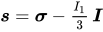
where 
A related set of quantities, (

where 

Another related set of widely used invariants is (

The 

The principal stresses and the Haigh-Westergaard coordinates are related by

A different definition of the Lode angle can also be found in the literature:
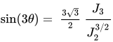
in which case the ordered principal stresses (where 
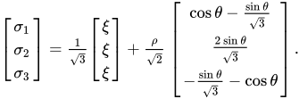
Note. It is incorrect (false) information that Chakrabarty did define shear stress mode angle with sin(3Teta). Chakrabarty adopted Lode parameter with opposite sign than it has in the original Lode paper from 1926, see Page 59, formula (3) in the book «Chakrabarty, Jagabanduhu; 2006, Theory of Plasticity: Third edition, Elsevier, Amsterdam.». Actually, Chakrabarty defined shear stress mode angle with -sin(3Teta) just like it did for the first time V.V. Novozhilov in his work from 1951, Novozhilov V.V., «O связи между напряжениями и деформациями в нелинейно упругой среде» (On relations between stresses and strains in non-linear elastic media), Прикладная математика и механика, 1951, p. 183-194; https://pmm.ipmnet.ru/ru/get/1951/15-2/183-194. The first work in which rational arguments and discussion is delivered why it is wise and useful to define shear stress mode angle with sin(.) function, regardless of the sign of the angle theta, is the Ziolkowski’s work «Parametrization of Cauchy Stress Tensor Treated as Autonomous Object Using Isotropy Angle and Skewness Angle» from 2022, https://et.ippt.pan.pl/index.php/et/article/view/2210, where it is elucidated that adopting definition of shear stress mode angle with sin(.) function physically means accepting pure shears as comparison reference states, and it is explained why it is very beneficial.


02Examples of yield surfaces
There are several different yield surfaces known in engineering, and those most popular are listed below.
Tresca yield surface
The Tresca yield criterion is taken to be the work of Henri Tresca. It is also known as the maximum shear stress theory (MSST) and the Tresca-Guest (TG) criterion. In terms of the principal stresses the Tresca criterion is expressed as

Where 

Figure 1 shows the Tresca-Guest yield surface in the three-dimensional space of principal stresses. It is a prism of six sides and having infinite length. This means that the material remains elastic when all three principal stresses are roughly equivalent (a hydrostatic pressure), no matter how much it is compressed or stretched. However, when one of the principal stresses becomes smaller (or larger) than the others the material is subject to shearing. In such situations, if the shear stress reaches the yield limit then the material enters the plastic domain. Figure 2 shows the Tresca-Guest yield surface in two-dimensional stress space, it is a cross section of the prism along the 
von Mises yield surface
The von Mises yield criterion is expressed in the principal stresses as

where
Figure 3 shows the von Mises yield surface in the three-dimensional space of principal stresses. It is a circular cylinder of infinite length with its axis inclined at equal angles to the three principal stresses. Figure 4 shows the von Mises yield surface in two-dimensional space compared with Tresca-Guest criterion. A cross section of the von Mises cylinder on the plane of
Burzyński-Yagn criterion
This criterion reformulated as the function of the hydrostatic nodes with the coordinates 

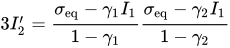
represents the general equation of a second order surface of revolution about the hydrostatic axis. Some special case are:
- cylinder
(Maxwell (1865), Huber (1904), von Mises (1913), Hencky (1924)),
- cone
(Botkin (1940), Drucker-Prager (1952), Mirolyubov (1953)),
- paraboloid
(Burzyński (1928), Balandin (1937), Torre (1947)),
- ellipsoid centered of symmetry plane
,
(Beltrami (1885)),
- ellipsoid centered of symmetry plane
with
(Schleicher (1926)),
- hyperboloid of two sheets
(Burzynski (1928), Yagn (1931)),
- hyperboloid of one sheet centered of symmetry plane
,
(Kuhn (1980))
- hyperboloid of one sheet
,
The relations compression-tension and torsion-tension can be computed to

The Poisson's ratios at tension and compression are obtained using


For ductile materials the restriction
![\nu _{+}^{\mathrm {in} }\in {\bigg [}\,0.48,\,{\frac {1}{2}}\,{\bigg ]}](https://wikimedia.org/api/rest_v1/media/math/render/svg/4b7c270b90d3c766fd6ecd9b7204e1622d9f7722)
is important. The application of rotationally symmetric criteria for brittle failure with
![\nu _{+}^{\mathrm {in} }\in ]-1,~\nu _{+}^{\mathrm {el} }\,]](https://wikimedia.org/api/rest_v1/media/math/render/svg/690096f2ce81fb70324e3cebefabb993721ed772)
has not been studied sufficiently.
The Burzyński-Yagn criterion is well suited for academic purposes. For practical applications, the third invariant of the deviator in the odd and even power should be introduced in the equation, e.g.:

Huber criterion
The Huber criterion consists of the Beltrami ellipsoid and a scaled von Mises cylinder in the principal stress space, see also
![3\,I_{2}'=\left\{{\begin{array}{ll}\displaystyle {\frac {\sigma _{\mathrm {eq} }-\gamma _{1}\,I_{1}}{1-\gamma _{1}}}\,{\frac {\sigma _{\mathrm {eq} }+\gamma _{1}\,I_{1}}{1+\gamma _{1}}},&I_{1}>0\\[1em]\displaystyle {\frac {\sigma _{\mathrm {eq} }}{1-\gamma _{1}}}\,{\frac {\sigma _{\mathrm {eq} }}{1+\gamma _{1}}},&I_{1}\leq 0\end{array}}\right.](https://wikimedia.org/api/rest_v1/media/math/render/svg/84e5badc1256fedb02c6e3bb4e32c3c04f455c74)
with 
- pressure-sensitive material behavior for
with
and
- pressure-insensitive material behavior for
with

The Huber criterion can be used as a yield surface with an empirical restriction for Poisson's ratio at tension ![\nu _{+}^{\mathrm {in} }\in [0.48,1/2]](https://wikimedia.org/api/rest_v1/media/math/render/svg/95b2a945c4242aba4b539c51f5dc7441fceda3b9)
![\gamma _{1}\in [0,0.1155]](https://wikimedia.org/api/rest_v1/media/math/render/svg/bee6b21ec154dddb4479a8f5fc3321c72ec824f4)
The modified Huber criterion, see also, cf.
![3\,I_{2}'=\left\{{\begin{array}{ll}\displaystyle {\frac {\sigma _{\mathrm {eq} }-\gamma _{1}\,I_{1}}{1-\gamma _{1}}}\,{\frac {\sigma _{\mathrm {eq} }-\gamma _{2}\,I_{1}}{1-\gamma _{2}}},&I_{1}>-d\,\sigma _{\mathrm {+} }\\[1em]\displaystyle {\frac {\sigma _{\mathrm {eq} }^{2}}{(1-\gamma _{1}-\gamma _{2})^{2}}},&I_{1}\leq -d\,\sigma _{\mathrm {+} }\end{array}}\right.](https://wikimedia.org/api/rest_v1/media/math/render/svg/7665d54a30d98465586f222a2ad1cf088bfd4d2a)
consists of the Schleicher ellipsoid with the restriction of Poisson's ratio at compression

and a cylinder with the 


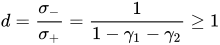
The modified Huber criterion can be better fitted to the measured data as the Huber criterion. For setting 


The Huber criterion and the modified Huber criterion should be preferred to the von Mises criterion since one obtains safer results in the region 

Mohr-Coulomb yield surface
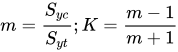
The Mohr-Coulomb yield (failure) criterion is similar to the Tresca criterion, with additional provisions for materials with different tensile and compressive yield strengths. This model is often used to model concrete, soil or granular materials. The Mohr-Coulomb yield criterion may be expressed as:

where
and the parameters 


Figure 5 shows Mohr-Coulomb yield surface in the three-dimensional space of principal stresses. It is a conical prism and 


Drucker-Prager yield surface
The Drucker-Prager yield criterion is similar to the von Mises yield criterion, with provisions for handling materials with differing tensile and compressive yield strengths. This criterion is most often used for concrete where both normal and shear stresses can determine failure. The Drucker-Prager yield criterion may be expressed as

where

and
Figure 7 shows Drucker-Prager yield surface in the three-dimensional space of principal stresses. It is a regular cone. Figure 8 shows Drucker-Prager yield surface in two-dimensional space. The elliptical elastic domain is a cross section of the cone on the plane of 

Bresler-Pister yield surface
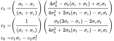
The Bresler-Pister yield criterion is an extension of the Drucker Prager yield criterion that uses three parameters, and has additional terms for materials that yield under hydrostatic compression. In terms of the principal stresses, this yield criterion may be expressed as
![S_{yc}={\tfrac {1}{\sqrt {2}}}\left[(\sigma _{1}-\sigma _{2})^{2}+(\sigma _{2}-\sigma _{3})^{2}+(\sigma _{3}-\sigma _{1})^{2}\right]^{1/2}-c_{0}-c_{1}~(\sigma _{1}+\sigma _{2}+\sigma _{3})-c_{2}~(\sigma _{1}+\sigma _{2}+\sigma _{3})^{2}](https://wikimedia.org/api/rest_v1/media/math/render/svg/168ce31fef86a9a05a75721a81e088c69edcf24f)
where 


Willam-Warnke yield surface
The Willam-Warnke yield criterion is a three-parameter smoothed version of the Mohr-Coulomb yield criterion that has similarities in form to the Drucker-Prager and Bresler-Pister yield criteria.
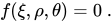
The yield criterion has the functional form

However, it is more commonly expressed in Haigh-Westergaard coordinates as
The cross-section of the surface when viewed along its axis is a smoothed triangle (unlike Mohr-Coulomb). The Willam-Warnke yield surface is convex and has unique and well defined first and second derivatives on every point of its surface. Therefore, the Willam-Warnke model is computationally robust and has been used for a variety of cohesive-frictional materials.
Podgórski and Rosendahl trigonometric yield surfaces
Normalized with respect to the uniaxial tensile stress 
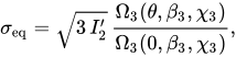
with the shape function of trigonal symmetry in the 
![\Omega _{3}(\theta ,\beta _{3},\chi _{3})=\cos \left[\displaystyle {\frac {1}{3}}\left(\pi \beta _{3}-\arccos[\,\sin(\chi _{3}\,{\frac {\pi }{2}})\,\!\cos 3\,\theta \,]\right)\right],\qquad \beta _{3}\in [0,\,1],\quad \chi _{3}\in [-1,\,1].](https://wikimedia.org/api/rest_v1/media/math/render/svg/31655f9e540e841ea6d966f7a0bdbe1fd6304b4a)
It contains the criteria of von Mises (circle in the ![\beta _{3}=[0,\,1]](https://wikimedia.org/api/rest_v1/media/math/render/svg/20634c0926a05259beda78f4e18b1ea6d38621be)


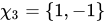


![\chi _{3}=[0,1]](https://wikimedia.org/api/rest_v1/media/math/render/svg/6b4456eca66f88480bde86583de8ac126d973ac4)
The Rosendahl criterion reads
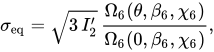
with the shape function of hexagonal symmetry in the
![\Omega _{6}(\theta ,\beta _{6},\chi _{6})=\cos \left[\displaystyle {\frac {1}{6}}\left(\pi \beta _{6}-\arccos[\,\sin(\chi _{6}\,{\frac {\pi }{2}})\,\!\cos 6\,\theta \,]\right)\right],\qquad \beta _{6}\in [0,\,1],\quad \chi _{6}\in [-1,\,1].](https://wikimedia.org/api/rest_v1/media/math/render/svg/e980c867fa1766fcc5a741ecf363e19c05a8bfe8)
It contains the criteria of von Mises (circle, ![\beta _{6}=[0,\,1]](https://wikimedia.org/api/rest_v1/media/math/render/svg/61f7b566943062df913486ad99edfa445fbb58a1)


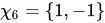


The criteria of Podgórski and Rosendahl describe single surfaces in principal stress space without any additional outer contours and plane intersections. Note that in order to avoid numerical issues the real part function 


A pressure-sensitive extension of the criteria can be obtained with the linear

which is sufficient for many applications, e.g. metals, cast iron, alloys, concrete, unreinforced polymers, etc.
Bigoni-Piccolroaz yield surface
The Bigoni-Piccolroaz yield criterion is a seven-parameter surface defined by

where 
![F(p)=\left\{{\begin{array}{ll}-Mp_{c}{\sqrt {(\phi -\phi ^{m})[2(1-\alpha )\phi +\alpha ]}},&\phi \in [0,1],\\+\infty ,&\phi \notin [0,1],\end{array}}\right.](https://wikimedia.org/api/rest_v1/media/math/render/svg/9948aa54df1e39ab115e425b19f088dff39beadc)

describing the pressure-sensitivity and 
![g(\theta )={\frac {1}{\cos[\beta {\frac {\pi }{6}}-{\frac {1}{3}}\cos ^{-1}(\gamma \cos 3\theta )]}},](https://wikimedia.org/api/rest_v1/media/math/render/svg/dba97f3c7548243d55f4c6736d862e34b31b04cb)
describing the Lode-dependence of yielding. The seven, non-negative material parameters:

define the shape of the meridian and deviatoric sections.
This criterion represents a smooth and convex surface, which is closed both in hydrostatic tension and compression and has a drop-like shape, particularly suited to describe frictional and granular materials. This criterion has also been generalized to the case of surfaces with corners.
Cosine Ansatz (Altenbach-Bolchoun-Kolupaev)
For the formulation of the strength criteria the stress angle
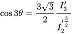
can be used.
The following criterion of isotropic material behavior

contains a number of other well-known less general criteria, provided suitable parameter values are chosen.
Parameters 


which follow from the convexity condition. A more precise formulation of the third constraints is proposed in.
Parameters 


The integer powers 


Barlat's Yield Surface
For the anisotropic materials, depending on the direction of the applied process (e.g., rolling) the mechanical properties vary and, therefore, using an anisotropic yield function is crucial. Since 1989 Frederic Barlat has developed a family of yield functions for constitutive modelling of plastic anisotropy. Among them, Yld2000-2D yield criteria has been applied for a wide range of sheet metals (e.g., aluminum alloys and advanced high-strength steels). The Yld2000-2D model is a non-quadratic type yield function based on two linear transformation of the stress tensor:
:
- where
is the effective stress. and
and
are the transformed matrices (by linear transformation C or L):
- where s is the deviatoric stress tensor.
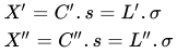
for principal values of X’ and X”, the model could be expressed as:

and:
![\left[{\begin{array}{*{20}{c}}{{L'}_{11}}\\{{L'}_{12}}\\{{L'}_{21}}\\{{L'}_{22}}\\{{L'}_{66}}\end{array}}\right]=\left[{\begin{array}{*{20}{c}}{2/3}&0&0\\{-1/3}&0&0\\0&{-1/3}&0\\0&{-2/3}&0\\0&0&1\end{array}}\right]\left[{\begin{array}{*{20}{c}}{\alpha _{1}}\\{\alpha _{2}}\\{\alpha _{7}}\end{array}}\right],\left[{\begin{array}{*{20}{c}}{{L''}_{11}}\\{{L''}_{12}}\\{{L''}_{21}}\\{{L''}_{22}}\\{{L''}_{66}}\end{array}}\right]=\left[{\begin{array}{*{20}{c}}{-2}&2&8&{-2}&0\\1&{-4}&{-4}&4&0\\4&{-4}&{-4}&4&0\\{-2}&8&2&{-2}&0\\0&0&0&0&1\end{array}}\right]\left[{\begin{array}{*{20}{c}}{\alpha _{3}}\\{\alpha _{4}}\\{\alpha _{5}}\\{\alpha _{6}}\\{\alpha _{8}}\end{array}}\right]](https://wikimedia.org/api/rest_v1/media/math/render/svg/4ad31d6027e7e5da286c1ec7579505cffa4c919c)
where 


Sources and credits
This article is adapted from the Wikipedia article “Yield surface”, written by its contributors and licensed under CC BY-SA 4.0. Fathomly has changed the layout, removed citation markers, navigation and maintenance notices, and adjusted punctuation. This adapted version is shared under the same license. For references, see the original article.
Images, from Wikimedia Commons:
- YieldSurface.svg by Bbanerje, CC BY-SA 3.0
- YieldSurfacerhoxitheta.svg by Bbanerje, CC BY-SA 3.0
- Tresca Guest Yield Surface 3D.png by Original uploader was Janek Kozicki at en.wikipedia, CC BY-SA 3.0
- Tresca Guest Yield Surface 2D.png by Janek Kozicki at en.wikipedia, CC BY-SA 3.0
- Mises Yield Surface 3D.png by Janek Kozicki at English Wikipedia, CC BY-SA 3.0
- Tresca stress 2D.png by Unknown author, Public domain
- Burzynski Huber F2 nuP0.jpg by VSchreimann, CC BY-SA 4.0
- MH Yield Surface 3D.png by Unknown author, CC BY-SA 3.0
Fathomly is not affiliated with or endorsed by the Wikimedia Foundation. Spotted a problem? Tell us.

