Encyclopedia

Weber modular function

Wikipedia contributorsAdapted for Fathomly · View authors

2 min read
Source updated September 17, 2025

In mathematics, the Weber modular functions are a family of three functions f, f₁, and f₂, studied by Heinrich Martin Weber.

01Definition

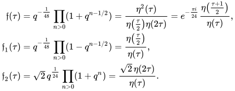
Let $q=e^{2\pi i\tau }$ where τ is an element of the upper half-plane. Then the Weber functions are

${\begin{aligned}{\mathfrak {f}}(\tau )&=q^{-{\frac {1}{48}}}\prod _{n>0}(1+q^{n-1/2})={\frac {\eta ^{2}(\tau )}{\eta {\big (}{\tfrac {\tau }{2}}{\big )}\eta (2\tau )}}=e^{-{\frac {\pi i}{24}}}{\frac {\eta {\big (}{\frac {\tau +1}{2}}{\big )}}{\eta (\tau )}},\\{\mathfrak {f}}_{1}(\tau )&=q^{-{\frac {1}{48}}}\prod _{n>0}(1-q^{n-1/2})={\frac {\eta {\big (}{\tfrac {\tau }{2}}{\big )}}{\eta (\tau )}},\\{\mathfrak {f}}_{2}(\tau )&={\sqrt {2}}\,q^{\frac {1}{24}}\prod _{n>0}(1+q^{n})={\frac {{\sqrt {2}}\,\eta (2\tau )}{\eta (\tau )}}.\end{aligned}}$

These are also the definitions in Duke's paper "Continued Fractions and Modular Functions". The function $\eta (\tau )$ is the Dedekind eta function and $(e^{2\pi i\tau })^{\alpha }$ should be interpreted as $e^{2\pi i\tau \alpha }$ . The descriptions as $\eta$ quotients immediately imply

${\mathfrak {f}}(\tau ){\mathfrak {f}}_{1}(\tau ){\mathfrak {f}}_{2}(\tau )={\sqrt {2}}.$

The transformation τ → , 1/τ fixes f and exchanges f₁ and f₂. So the 3-dimensional complex vector space with basis f, f₁ and f₂ is acted on by the group SL₂(Z).

02Alternative infinite product

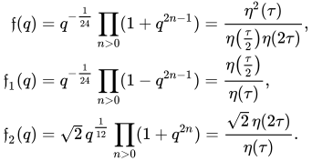
Alternatively, let $q=e^{\pi i\tau }$ be the nome,

${\begin{aligned}{\mathfrak {f}}(q)&=q^{-{\frac {1}{24}}}\prod _{n>0}(1+q^{2n-1})={\frac {\eta ^{2}(\tau )}{\eta {\big (}{\tfrac {\tau }{2}}{\big )}\eta (2\tau )}},\\{\mathfrak {f}}_{1}(q)&=q^{-{\frac {1}{24}}}\prod _{n>0}(1-q^{2n-1})={\frac {\eta {\big (}{\tfrac {\tau }{2}}{\big )}}{\eta (\tau )}},\\{\mathfrak {f}}_{2}(q)&={\sqrt {2}}\,q^{\frac {1}{12}}\prod _{n>0}(1+q^{2n})={\frac {{\sqrt {2}}\,\eta (2\tau )}{\eta (\tau )}}.\end{aligned}}$

The form of the infinite product has slightly changed. But since the eta quotients remain the same, then ${\mathfrak {f}}_{i}(\tau )={\mathfrak {f}}_{i}(q)$ as long as the second uses the nome $q=e^{\pi i\tau }$ . The utility of the second form is to show connections and consistent notation with the Ramanujan G- and g-functions and the Jacobi theta functions, both of which conventionally uses the nome.

03Relation to the Ramanujan G and g functions

Still employing the nome $q=e^{\pi i\tau }$ , define the Ramanujan G- and g-functions as

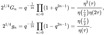
${\begin{aligned}2^{1/4}G_{n}&=q^{-{\frac {1}{24}}}\prod _{n>0}(1+q^{2n-1})={\frac {\eta ^{2}(\tau )}{\eta {\big (}{\tfrac {\tau }{2}}{\big )}\eta (2\tau )}},\\2^{1/4}g_{n}&=q^{-{\frac {1}{24}}}\prod _{n>0}(1-q^{2n-1})={\frac {\eta {\big (}{\tfrac {\tau }{2}}{\big )}}{\eta (\tau )}}.\end{aligned}}$

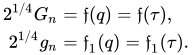
The eta quotients make their connection to the first two Weber functions immediately apparent. In the nome, assume $\tau ={\sqrt {-n}}.$ Then,

${\begin{aligned}2^{1/4}G_{n}&={\mathfrak {f}}(q)={\mathfrak {f}}(\tau ),\\2^{1/4}g_{n}&={\mathfrak {f}}_{1}(q)={\mathfrak {f}}_{1}(\tau ).\end{aligned}}$

Ramanujan found many relations between $G_{n}$ and $g_{n}$ which implies similar relations between ${\mathfrak {f}}(q)$ and ${\mathfrak {f}}_{1}(q)$ . For example, his identity,

$(G_{n}^{8}-g_{n}^{8})(G_{n}\,g_{n})^{8}={\tfrac {1}{4}},$

leads to

${\big [}{\mathfrak {f}}^{8}(q)-{\mathfrak {f}}_{1}^{8}(q){\big ]}{\big [}{\mathfrak {f}}(q)\,{\mathfrak {f}}_{1}(q){\big ]}^{8}={\big [}{\sqrt {2}}{\big ]}^{8}.$

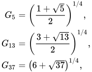
For many values of n, Ramanujan also tabulated $G_{n}$ for odd n, and $g_{n}$ for even n. This automatically gives many explicit evaluations of ${\mathfrak {f}}(q)$ and ${\mathfrak {f}}_{1}(q)$ . For example, using $\tau ={\sqrt {-5}},\,{\sqrt {-13}},\,{\sqrt {-37}}$ , which are some of the square-free discriminants with class number 2,

${\begin{aligned}G_{5}&=\left({\frac {1+{\sqrt {5}}}{2}}\right)^{1/4},\\G_{13}&=\left({\frac {3+{\sqrt {13}}}{2}}\right)^{1/4},\\G_{37}&=\left(6+{\sqrt {37}}\right)^{1/4},\end{aligned}}$

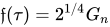
and one can easily get ${\mathfrak {f}}(\tau )=2^{1/4}G_{n}$ from these, as well as the more complicated examples found in Ramanujan's Notebooks.

04Relation to Jacobi theta functions

The argument of the classical Jacobi theta functions is traditionally the nome $q=e^{\pi i\tau },$

${\begin{aligned}\vartheta _{10}(0;\tau )&=\theta _{2}(q)=\sum _{n=-\infty }^{\infty }q^{(n+1/2)^{2}}={\frac {2\eta ^{2}(2\tau )}{\eta (\tau )}},\\[2pt]\vartheta _{00}(0;\tau )&=\theta _{3}(q)=\sum _{n=-\infty }^{\infty }q^{n^{2}}\;=\;{\frac {\eta ^{5}(\tau )}{\eta ^{2}\left({\frac {\tau }{2}}\right)\eta ^{2}(2\tau )}}={\frac {\eta ^{2}\left({\frac {\tau +1}{2}}\right)}{\eta (\tau +1)}},\\[3pt]\vartheta _{01}(0;\tau )&=\theta _{4}(q)=\sum _{n=-\infty }^{\infty }(-1)^{n}q^{n^{2}}={\frac {\eta ^{2}\left({\frac {\tau }{2}}\right)}{\eta (\tau )}}.\end{aligned}}$

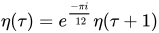
Dividing them by $\eta (\tau )$ , and also noting that $\eta (\tau )=e^{\frac {-\pi i}{\,12}}\eta (\tau +1)$ , then they are just squares of the Weber functions ${\mathfrak {f}}_{i}(q)$

${\begin{aligned}{\frac {\theta _{2}(q)}{\eta (\tau )}}&={\mathfrak {f}}_{2}(q)^{2},\\[4pt]{\frac {\theta _{4}(q)}{\eta (\tau )}}&={\mathfrak {f}}_{1}(q)^{2},\\[4pt]{\frac {\theta _{3}(q)}{\eta (\tau )}}&={\mathfrak {f}}(q)^{2},\end{aligned}}$

with even-subscript theta functions purposely listed first. Using the well-known Jacobi identity with even subscripts on the LHS,

$\theta _{2}(q)^{4}+\theta _{4}(q)^{4}=\theta _{3}(q)^{4};$

therefore,

${\mathfrak {f}}_{2}(q)^{8}+{\mathfrak {f}}_{1}(q)^{8}={\mathfrak {f}}(q)^{8}.$

05Relation to j-function

The three roots of the cubic equation

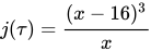
$j(\tau )={\frac {(x-16)^{3}}{x}}$

where j(τ) is the j-function are given by $x_{i}={\mathfrak {f}}(\tau )^{24},-{\mathfrak {f}}_{1}(\tau )^{24},-{\mathfrak {f}}_{2}(\tau )^{24}$ . Also, since,

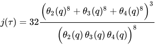
$j(\tau )=32{\frac {{\Big (}\theta _{2}(q)^{8}+\theta _{3}(q)^{8}+\theta _{4}(q)^{8}{\Big )}^{3}}{{\Big (}\theta _{2}(q)\,\theta _{3}(q)\,\theta _{4}(q){\Big )}^{8}}}$

and using the definitions of the Weber functions in terms of the Jacobi theta functions, plus the fact that ${\mathfrak {f}}_{2}(q)^{2}\,{\mathfrak {f}}_{1}(q)^{2}\,{\mathfrak {f}}(q)^{2}={\frac {\theta _{2}(q)}{\eta (\tau )}}{\frac {\theta _{4}(q)}{\eta (\tau )}}{\frac {\theta _{3}(q)}{\eta (\tau )}}=2$ , then

$j(\tau )=\left({\frac {{\mathfrak {f}}(\tau )^{16}+{\mathfrak {f}}_{1}(\tau )^{16}+{\mathfrak {f}}_{2}(\tau )^{16}}{2}}\right)^{3}=\left({\frac {{\mathfrak {f}}(q)^{16}+{\mathfrak {f}}_{1}(q)^{16}+{\mathfrak {f}}_{2}(q)^{16}}{2}}\right)^{3}$

since ${\mathfrak {f}}_{i}(\tau )={\mathfrak {f}}_{i}(q)$ and have the same formulas in terms of the Dedekind eta function $\eta (\tau )$ .

Watch videos about Weber modular functionExplainers and documentaries on YouTube (opens in a new tab)

Sources and credits

This article is adapted from the Wikipedia article “Weber modular function”, written by its contributors and licensed under CC BY-SA 4.0. Fathomly has changed the layout, removed citation markers, navigation and maintenance notices, and adjusted punctuation. This adapted version is shared under the same license. For references, see the original article.

Fathomly is not affiliated with or endorsed by the Wikimedia Foundation. Spotted a problem? Tell us.