Encyclopedia

Vector-radix FFT algorithm

Multidimensional fast Fourier transform algorithm

Wikipedia contributorsAdapted for Fathomly · View authors

3 min read
Source updated November 6, 2025

The vector-radix FFT algorithm, is a multidimensional fast Fourier transform (FFT) algorithm, which is a generalization of the ordinary Cooley-Tukey FFT algorithm that divides the transform dimensions by arbitrary radices. It breaks a multidimensional (MD) discrete Fourier transform (DFT) down into successively smaller MD DFTs until, ultimately, only trivial MD DFTs need to be evaluated.

The most common multidimensional FFT algorithm is the row-column algorithm, which means transforming the array first in one index and then in the other, see more in FFT. Then a radix-2 direct 2-D FFT has been developed, and it can eliminate 25% of the multiplies as compared to the conventional row-column approach. And this algorithm has been extended to rectangular arrays and arbitrary radices, which is the general vector-radix algorithm.

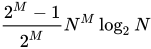
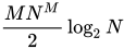
Vector-radix FFT algorithm can reduce the number of complex multiplications significantly, compared to row-vector algorithm. For example, for a $N^{M}$ element matrix (M dimensions, and size N on each dimension), the number of complex multiples of vector-radix FFT algorithm for radix-2 is ${\frac {2^{M}-1}{2^{M}}}N^{M}\log _{2}N$ , meanwhile, for row-column algorithm, it is ${\frac {MN^{M}}{2}}\log _{2}N$ . And generally, even larger savings in multiplies are obtained when this algorithm is operated on larger radices and on higher dimensional arrays.

Overall, the vector-radix algorithm significantly reduces the structural complexity of the traditional DFT having a better indexing scheme, at the expense of a slight increase in arithmetic operations. So this algorithm is widely used for many applications in engineering, science, and mathematics, for example, implementations in image processing, and high speed FFT processor designing.

012-D DIT case

As with the Cooley-Tukey FFT algorithm, the two dimensional vector-radix FFT is derived by decomposing the regular 2-D DFT into sums of smaller DFT's multiplied by "twiddle" factors.

A decimation-in-time (DIT) algorithm means the decomposition is based on time domain $x$ , see more in Cooley-Tukey FFT algorithm.

We suppose the 2-D DFT is defined

$X(k_{1},k_{2})=\sum _{n_{1}=0}^{N_{1}-1}\sum _{n_{2}=0}^{N_{2}-1}x[n_{1},n_{2}]\cdot W_{N_{1}}^{k_{1}n_{1}}W_{N_{2}}^{k_{2}n_{2}},$

where $k_{1}=0,\dots ,N_{1}-1$ , and $k_{2}=0,\dots ,N_{2}-1$ , and $x[n_{1},n_{2}]$ is an $N_{1}\times N_{2}$ matrix, and $W_{N}=\exp(-j2\pi /N)$ .

For simplicity, let us assume that $N_{1}=N_{2}=N$ , and the radix- $(r\times r)$ is such that $N/r$ is an integer.

Using the change of variables:

$n_{i}=rp_{i}+q_{i}$ , where $p_{i}=0,\ldots ,(N/r)-1;q_{i}=0,\ldots ,r-1;$
$k_{i}=u_{i}+v_{i}N/r$ , where $u_{i}=0,\ldots ,(N/r)-1;v_{i}=0,\ldots ,r-1;$

where $i=1$ or $2$ , then the two dimensional DFT can be written as:

$X(u_{1}+v_{1}N/r,u_{2}+v_{2}N/r)=\sum _{q_{1}=0}^{r-1}\sum _{q_{2}=0}^{r-1}\left[\sum _{p_{1}=0}^{N/r-1}\sum _{p_{2}=0}^{N/r-1}x[rp_{1}+q_{1},rp_{2}+q_{2}]W_{N/r}^{p_{1}u_{1}}W_{N/r}^{p_{2}u_{2}}\right]\cdot W_{N}^{q_{1}u_{1}+q_{2}u_{2}}W_{r}^{q_{1}v_{1}}W_{r}^{q_{2}v_{2}},$

The equation above defines the basic structure of the 2-D DIT radix- $(r\times r)$ "butterfly". (See 1-D "butterfly" in Cooley-Tukey FFT algorithm)

When $r=2$ , the equation can be broken into four summations, and this leads to:

$X(k_{1},k_{2})=S_{00}(k_{1},k_{2})+S_{01}(k_{1},k_{2})W_{N}^{k_{2}}+S_{10}(k_{1},k_{2})W_{N}^{k_{1}}+S_{11}(k_{1},k_{2})W_{N}^{k_{1}+k_{2}}$ for $0\leq k_{1},k_{2}<{\frac {N}{2}}$ ,

where $S_{ij}(k_{1},k_{2})=\sum _{n_{1}=0}^{N/2-1}\sum _{n_{2}=0}^{N/2-1}x[2n_{1}+i,2n_{2}+j]\cdot W_{N/2}^{n_{1}k_{1}}W_{N/2}^{n_{2}k_{2}}$ .

The $S_{ij}$ can be viewed as the $N/2$ -dimensional DFT, each over a subset of the original sample:

$S_{00}$ is the DFT over those samples of $x$ for which both $n_{1}$ and $n_{2}$ are even;
$S_{01}$ is the DFT over the samples for which $n_{1}$ is even and $n_{2}$ is odd;
$S_{10}$ is the DFT over the samples for which $n_{1}$ is odd and $n_{2}$ is even;
$S_{11}$ is the DFT over the samples for which both $n_{1}$ and $n_{2}$ are odd.

Thanks to the periodicity of the complex exponential, we can obtain the following additional identities, valid for $0\leq k_{1},k_{2}<{\frac {N}{2}}$ :

$X{\biggl (}k_{1}+{\frac {N}{2}},k_{2}{\biggr )}=S_{00}(k_{1},k_{2})+S_{01}(k_{1},k_{2})W_{N}^{k_{2}}-S_{10}(k_{1},k_{2})W_{N}^{k_{1}}-S_{11}(k_{1},k_{2})W_{N}^{k_{1}+k_{2}}$ ;
$X{\biggl (}k_{1},k_{2}+{\frac {N}{2}}{\biggr )}=S_{00}(k_{1},k_{2})-S_{01}(k_{1},k_{2})W_{N}^{k_{2}}+S_{10}(k_{1},k_{2})W_{N}^{k_{1}}-S_{11}(k_{1},k_{2})W_{N}^{k_{1}+k_{2}}$ ;
$X{\biggl (}k_{1}+{\frac {N}{2}},k_{2}+{\frac {N}{2}}{\biggr )}=S_{00}(k_{1},k_{2})-S_{01}(k_{1},k_{2})W_{N}^{k_{2}}-S_{10}(k_{1},k_{2})W_{N}^{k_{1}}+S_{11}(k_{1},k_{2})W_{N}^{k_{1}+k_{2}}$ .

022-D DIF case

Similarly, a decimation-in-frequency (DIF, also called the Sande-Tukey algorithm) algorithm means the decomposition is based on frequency domain $X$ , see more in Cooley-Tukey FFT algorithm.

Using the change of variables:

$n_{i}=p_{i}+q_{i}N/r$ , where $p_{i}=0,\ldots ,(N/r)-1;q_{i}=0,\ldots ,r-1;$
$k_{i}=ru_{i}+v_{i}$ , where $u_{i}=0,\ldots ,(N/r)-1;v_{i}=0,\ldots ,r-1;$

where $i=1$ or $2$ , and the DFT equation can be written as:

$X(ru_{1}+v_{1},ru_{2}+v_{2})=\sum _{p_{1}=0}^{N/r-1}\sum _{p_{2}=0}^{N/r-1}\left[\sum _{q_{1}=0}^{r-1}\sum _{q_{2}=0}^{r-1}x[p_{1}+q_{1}N/r,p_{2}+q_{2}N/r]W_{r}^{q_{1}v_{1}}W_{r}^{q_{2}v_{2}}\right]\cdot W_{N}^{p_{1}v_{1}+p_{2}v_{2}}W_{N/r}^{p_{1}u_{1}}W_{N/r}^{p_{2}u_{2}},$

03Other approaches

The split-radix FFT algorithm has been proved to be a useful method for 1-D DFT. And this method has been applied to the vector-radix FFT to obtain a split vector-radix FFT.

In conventional 2-D vector-radix algorithm, we decompose the indices $k_{1},k_{2}$ into 4 groups:

${\begin{array}{lcl}X(2k_{1},2k_{2})&:&{\text{even-even}}\\X(2k_{1},2k_{2}+1)&:&{\text{even-odd}}\\X(2k_{1}+1,2k_{2})&:&{\text{odd-even}}\\X(2k_{1}+1,2k_{2}+1)&:&{\text{odd-odd}}\end{array}}$

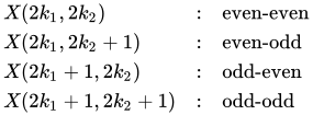
By the split vector-radix algorithm, the first three groups remain unchanged, the fourth odd-odd group is further decomposed into another four sub-groups, and seven groups in total:

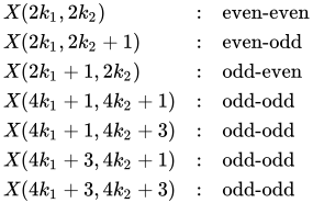
${\begin{array}{lcl}X(2k_{1},2k_{2})&:&{\text{even-even}}\\X(2k_{1},2k_{2}+1)&:&{\text{even-odd}}\\X(2k_{1}+1,2k_{2})&:&{\text{odd-even}}\\X(4k_{1}+1,4k_{2}+1)&:&{\text{odd-odd}}\\X(4k_{1}+1,4k_{2}+3)&:&{\text{odd-odd}}\\X(4k_{1}+3,4k_{2}+1)&:&{\text{odd-odd}}\\X(4k_{1}+3,4k_{2}+3)&:&{\text{odd-odd}}\end{array}}$

That means the fourth term in 2-D DIT radix- $(2\times 2)$ equation, $S_{11}(k_{1},k_{2})W_{N}^{k_{1}+k_{2}}$ becomes:

$A_{11}(k_{1},k_{2})W_{N}^{k_{1}+k_{2}}+A_{13}(k_{1},k_{2})W_{N}^{k_{1}+3k_{2}}+A_{31}(k_{1},k_{2})W_{N}^{3k_{1}+k_{2}}+A_{33}(k_{1},k_{2})W_{N}^{3(k_{1}+k_{2})},$

where $A_{ij}(k_{1},k_{2})=\sum _{n_{1}=0}^{N/4-1}\sum _{n_{2}=0}^{N/4-1}x[4n_{1}+i,4n_{2}+j]\cdot W_{N/4}^{n_{1}k_{1}}W_{N/4}^{n_{2}k_{2}}$

The 2-D N by N DFT is then obtained by successive use of the above decomposition, up to the last stage.

It has been shown that the split vector radix algorithm has saved about 30% of the complex multiplications and about the same number of the complex additions for typical $1024\times 1024$ array, compared with the vector-radix algorithm.

Watch videos about Vector-radix FFT algorithmExplainers and documentaries on YouTube (opens in a new tab)

Sources and credits

This article is adapted from the Wikipedia article “Vector-radix FFT algorithm”, written by its contributors and licensed under CC BY-SA 4.0. Fathomly has changed the layout, removed citation markers, navigation and maintenance notices, and adjusted punctuation. This adapted version is shared under the same license. For references, see the original article.

Images, from Wikimedia Commons:

2x2 radix butterfly diagram.svg by Spiritual Directive, CC BY-SA 4.0

Fathomly is not affiliated with or endorsed by the Wikimedia Foundation. Spotted a problem? Tell us.