True anomaly
Parameter of Keplerian orbits

In celestial mechanics, true anomaly is an angular parameter that defines the position of a body moving along a Keplerian orbit. It is the angle between the direction of periapsis and the current position of the body, as seen from the main focus of the ellipse (the point around which the object orbits).
The true anomaly is usually denoted by the Greek letters ν or θ, or the Latin letter f, and is usually restricted to the range 0-360° (0-2π rad).
The true anomaly f is one of three angular parameters (anomalies) that can be used to define a position along an orbit, the other two being the eccentric anomaly and the mean anomaly.
01Etymology
The term "anomaly" originally referred to the irregular movements of planets. Over time, that phrase evolved to refer to the general angular location of a planet around its orbit. The word true was added to refer to the actual angular location as opposed to other estimations of calculations of angular locations, for example mean anomaly.
02Formulas
From state vectors
For elliptic orbits, the true anomaly ν can be calculated from orbital state vectors as:
- (if r ⋅ v < 0 then replace ν by 2π − ν)
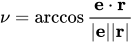
where:
- v is the orbital velocity vector of the orbiting body,
- e is the eccentricity vector,
- r is the orbital position vector (segment FP in the figure) of the orbiting body.
Circular orbit
For circular orbits the true anomaly is undefined, because circular orbits do not have a uniquely determined periapsis. Instead the argument of latitude u is used:
- (if rz < 0 then replace u by 2π − u)
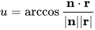
where:
- n is a vector pointing towards the ascending node (i.e. the z-component of n is zero).
- rz is the z-component of the orbital position vector r
Circular orbit with zero inclination
For circular orbits with zero inclination the argument of latitude is also undefined, because there is no uniquely determined line of nodes. One uses the true longitude instead:
- (if vx > 0 then replace l by 2π − l)
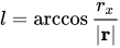
where:
- rx is the x-component of the orbital position vector r
- vx is the x-component of the orbital velocity vector v.
From the eccentric anomaly
The relation between the true anomaly ν and the eccentric anomaly 
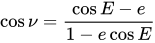
or using the sine and tangent:
![{\begin{aligned}\sin {\nu }&={{{\sqrt {1-e^{2}\,}}\sin {E}} \over {1-e\cos {E}}}\\[4pt]\tan {\nu }={{\sin {\nu }} \over {\cos {\nu }}}&={{{\sqrt {1-e^{2}\,}}\sin {E}} \over {\cos {E}-e}}\end{aligned}}](https://wikimedia.org/api/rest_v1/media/math/render/svg/e78fa556ab9265fb1281a7a87ae21f9e290615a9)
or equivalently:
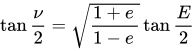
so

Alternatively, a form of this equation was derived by R. Broucke and P. Cefola that avoids numerical issues when the arguments are near 


where
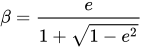
so

From the mean anomaly
The true anomaly can be calculated directly from the mean anomaly 
![\nu =M+2\sum _{k=1}^{\infty }{\frac {1}{k}}\left[\sum _{n=-\infty }^{\infty }J_{n}(-ke)\beta ^{|k+n|}\right]\sin {kM}](https://wikimedia.org/api/rest_v1/media/math/render/svg/e62a3776e7b4fb5f247edb91b14c857e93fc8fd9)
with Bessel functions 
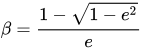
Omitting all terms of order 


Note that for reasons of accuracy this approximation is usually limited to orbits where the eccentricity 
The expression 
Radius from true anomaly
The radius (distance between the focus of attraction and the orbiting body) is related to the true anomaly by the formula

where a is the orbit's semi-major axis.
In celestial mechanics, Projective anomaly is an angular parameter that defines the position of a body moving along a Keplerian orbit. It is the angle between the direction of periapsis and the current position of the body in the projective space.
The projective anomaly is usually denoted by 

The projective anomaly
In the projective geometry, circles, ellipses, parabolae, and hyperbolae are treated as the same kind of quadratic curves.
03Projective parameters and projective anomaly
An orbit type is classified by two project parameters 

- circular orbit
- elliptic orbit
- parabolic orbit
- hyperbolic orbit
- linear orbit
- imaginary orbit


where



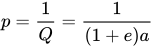
where 

Position and heliocentric distance of the planet 


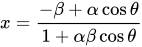
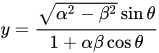
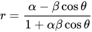
04Kepler's equation
The projective anomaly 
- Case :
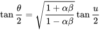

- case :

- case :
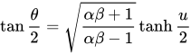

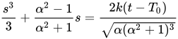
The above equations are called Kepler's equation.
05Generalized anomaly
For arbitrary constant 


The eccentric anomaly, the true anomaly, and the projective anomaly are the cases of 


- Sato, I., "A New Anomaly of Keplerian Motion", Astronomical Journal Vol.116, pp. 2038-3039, (1997)
Sources and credits
This article is adapted from the Wikipedia article “True anomaly”, written by its contributors and licensed under CC BY-SA 4.0. Fathomly has changed the layout, removed citation markers, navigation and maintenance notices, and adjusted punctuation. This adapted version is shared under the same license. For references, see the original article.
Images, from Wikimedia Commons:
- Eccentric and True Anomaly.svg by CheCheDaWaff, CC BY-SA 4.0
Fathomly is not affiliated with or endorsed by the Wikimedia Foundation. Spotted a problem? Tell us.

