Encyclopedia

Multilinear multiplication

Wikipedia contributorsAdapted for Fathomly · View authors

2 min read
Source updated September 14, 2026

In multilinear algebra, applying a map that is the tensor product of linear maps to a tensor is called a multilinear multiplication.

01Abstract definition

Let $F$ be a field of characteristic zero, such as $\mathbb {R}$ or $\mathbb {C}$ . Let $V_{k}$ be a finite-dimensional vector space over $F$ , and let ${\mathcal {A}}\in V_{1}\otimes V_{2}\otimes \cdots \otimes V_{d}$ be an order-d simple tensor, i.e., there exist some vectors $\mathbf {v} _{k}\in V_{k}$ such that ${\mathcal {A}}=\mathbf {v} _{1}\otimes \mathbf {v} _{2}\otimes \cdots \otimes \mathbf {v} _{d}$ . If we are given a collection of linear maps $A_{k}:V_{k}\to W_{k}$ , then the multilinear multiplication of ${\mathcal {A}}$ with $(A_{1},A_{2},\ldots ,A_{d})$ is defined as the action on ${\mathcal {A}}$ of the tensor product of these linear maps, namely

${\begin{aligned}A_{1}\otimes A_{2}\otimes \cdots \otimes A_{d}:V_{1}\otimes V_{2}\otimes \cdots \otimes V_{d}&\to W_{1}\otimes W_{2}\otimes \cdots \otimes W_{d},\\\mathbf {v} _{1}\otimes \mathbf {v} _{2}\otimes \cdots \otimes \mathbf {v} _{d}&\mapsto A_{1}(\mathbf {v} _{1})\otimes A_{2}(\mathbf {v} _{2})\otimes \cdots \otimes A_{d}(\mathbf {v} _{d})\end{aligned}}$

Since the tensor product of linear maps is itself a linear map, and because every tensor admits a tensor rank decomposition, the above expression extends linearly to all tensors. That is, for a general tensor ${\mathcal {A}}\in V_{1}\otimes V_{2}\otimes \cdots \otimes V_{d}$ , the multilinear multiplication is

${\begin{aligned}&{\mathcal {B}}:=(A_{1}\otimes A_{2}\otimes \cdots \otimes A_{d})({\mathcal {A}})\\[4pt]={}&(A_{1}\otimes A_{2}\otimes \cdots \otimes A_{d})\left(\sum _{i=1}^{r}\mathbf {a} _{i}^{1}\otimes \mathbf {a} _{i}^{2}\otimes \cdots \otimes \mathbf {a} _{i}^{d}\right)\\[5pt]={}&\sum _{i=1}^{r}A_{1}(\mathbf {a} _{i}^{1})\otimes A_{2}(\mathbf {a} _{i}^{2})\otimes \cdots \otimes A_{d}(\mathbf {a} _{i}^{d})\end{aligned}}$

where ${\textstyle {\mathcal {A}}=\sum _{i=1}^{r}\mathbf {a} _{i}^{1}\otimes \mathbf {a} _{i}^{2}\otimes \cdots \otimes \mathbf {a} _{i}^{d}$ with $\mathbf {a} _{i}^{k}\in V_{k}$ is one of ${\mathcal {A}}$ 's tensor rank decompositions. The validity of the above expression is not limited to a tensor rank decomposition; in fact, it is valid for any expression of ${\mathcal {A}}$ as a linear combination of pure tensors, which follows from the universal property of the tensor product.

It is standard to use the following shorthand notations in the literature for multilinear multiplications: $(A_{1},A_{2},\ldots ,A_{d})\cdot {\mathcal {A}}:=(A_{1}\otimes A_{2}\otimes \cdots \otimes A_{d})({\mathcal {A}})$ and $A_{k}\cdot _{k}{\mathcal {A}}:=(\operatorname {Id} _{V_{1}},\ldots ,\operatorname {Id} _{V_{k-1}},A_{k},\operatorname {Id} _{V_{k+1}},\ldots ,\operatorname {Id} _{V_{d}})\cdot {\mathcal {A}},$ where $\operatorname {Id} _{V_{k}}:V_{k}\to V_{k}$ is the identity operator.

02Definition in coordinates

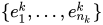
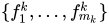
In computational multilinear algebra it is conventional to work in coordinates. Assume that an inner product is fixed on $V_{k}$ and let $V_{k}^{*}$ denote the dual vector space of $V_{k}$ . Let $\{e_{1}^{k},\ldots ,e_{n_{k}}^{k}\}$ be a basis for $V_{k}$ , let $\{(e_{1}^{k})^{*},\ldots ,(e_{n_{k}}^{k})^{*}\}$ be the dual basis, and let $\{f_{1}^{k},\ldots ,f_{m_{k}}^{k}\}$ be a basis for $W_{k}$ . The linear map ${\textstyle M_{k}=\sum _{i=1}^{m_{k}}\sum _{j=1}^{n_{k}}m_{i,j}^{(k)}f_{i}^{k}\otimes (e_{j}^{k})^{*}$ is then represented by the matrix ${\widehat {M}}_{k}=[m_{i,j}^{(k)}]\in F^{m_{k}\times n_{k}}$ . Likewise, with respect to the standard tensor product basis $\{e_{j_{1}}^{1}\otimes e_{j_{2}}^{2}\otimes \cdots \otimes e_{j_{d}}^{d}\}_{j_{1},j_{2},\ldots ,j_{d}}$ , the abstract tensor ${\mathcal {A}}=\sum _{j_{1}=1}^{n_{1}}\sum _{j_{2}=1}^{n_{2}}\cdots \sum _{j_{d}=1}^{n_{d}}a_{j_{1},j_{2},\ldots ,j_{d}}e_{j_{1}}^{1}\otimes e_{j_{2}}^{2}\otimes \cdots \otimes e_{j_{d}}^{d}$ is represented by the multidimensional array ${\widehat {\mathcal {A}}}=[a_{j_{1},j_{2},\ldots ,j_{d}}]\in F^{n_{1}\times n_{2}\times \cdots \times n_{d}}$ . Observe that ${\widehat {\mathcal {A}}}=\sum _{j_{1}=1}^{n_{1}}\sum _{j_{2}=1}^{n_{2}}\cdots \sum _{j_{d}=1}^{n_{d}}a_{j_{1},j_{2},\ldots ,j_{d}}\mathbf {e} _{j_{1}}^{1}\otimes \mathbf {e} _{j_{2}}^{2}\otimes \cdots \otimes \mathbf {e} _{j_{d}}^{d},$

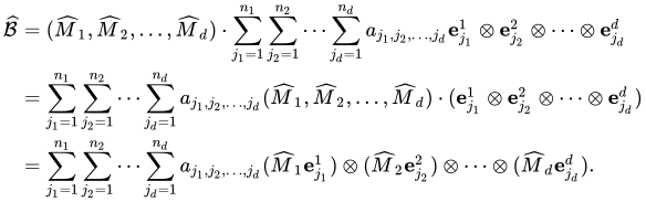
where $\mathbf {e} _{j}^{k}\in F^{n_{k}}$ is the jth standard basis vector of $F^{n_{k}}$ and the tensor product of vectors is the affine Segre map $\otimes :(\mathbf {v} ^{(1)},\mathbf {v} ^{(2)},\ldots ,\mathbf {v} ^{(d)})\mapsto [v_{i_{1}}^{(1)}v_{i_{2}}^{(2)}\cdots v_{i_{d}}^{(d)}]_{i_{1},i_{2},\ldots ,i_{d}}$ . It follows from the above choices of bases that the multilinear multiplication ${\mathcal {B}}=(M_{1},M_{2},\ldots ,M_{d})\cdot {\mathcal {A}}$ becomes

${\begin{aligned}{\widehat {\mathcal {B}}}&=({\widehat {M}}_{1},{\widehat {M}}_{2},\ldots ,{\widehat {M}}_{d})\cdot \sum _{j_{1}=1}^{n_{1}}\sum _{j_{2}=1}^{n_{2}}\cdots \sum _{j_{d}=1}^{n_{d}}a_{j_{1},j_{2},\ldots ,j_{d}}\mathbf {e} _{j_{1}}^{1}\otimes \mathbf {e} _{j_{2}}^{2}\otimes \cdots \otimes \mathbf {e} _{j_{d}}^{d}\\&=\sum _{j_{1}=1}^{n_{1}}\sum _{j_{2}=1}^{n_{2}}\cdots \sum _{j_{d}=1}^{n_{d}}a_{j_{1},j_{2},\ldots ,j_{d}}({\widehat {M}}_{1},{\widehat {M}}_{2},\ldots ,{\widehat {M}}_{d})\cdot (\mathbf {e} _{j_{1}}^{1}\otimes \mathbf {e} _{j_{2}}^{2}\otimes \cdots \otimes \mathbf {e} _{j_{d}}^{d})\\&=\sum _{j_{1}=1}^{n_{1}}\sum _{j_{2}=1}^{n_{2}}\cdots \sum _{j_{d}=1}^{n_{d}}a_{j_{1},j_{2},\ldots ,j_{d}}({\widehat {M}}_{1}\mathbf {e} _{j_{1}}^{1})\otimes ({\widehat {M}}_{2}\mathbf {e} _{j_{2}}^{2})\otimes \cdots \otimes ({\widehat {M}}_{d}\mathbf {e} _{j_{d}}^{d}).\end{aligned}}$

The resulting tensor ${\widehat {\mathcal {B}}}$ lives in $F^{m_{1}\times m_{2}\times \cdots \times m_{d}}$ .

Element-wise definition

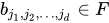
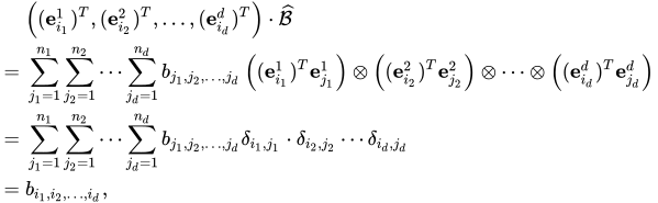
From the above expression, an element-wise definition of the multilinear multiplication is obtained. Indeed, since ${\widehat {\mathcal {B}}}$ is a multidimensional array, it may be expressed as ${\widehat {\mathcal {B}}}=\sum _{j_{1}=1}^{n_{1}}\sum _{j_{2}=1}^{n_{2}}\cdots \sum _{j_{d}=1}^{n_{d}}b_{j_{1},j_{2},\ldots ,j_{d}}\mathbf {e} _{j_{1}}^{1}\otimes \mathbf {e} _{j_{2}}^{2}\otimes \cdots \otimes \mathbf {e} _{j_{d}}^{d},$ where $b_{j_{1},j_{2},\ldots ,j_{d}}\in F$ are the coefficients. Then it follows from the above formulae that

${\begin{aligned}&\left((\mathbf {e} _{i_{1}}^{1})^{T},(\mathbf {e} _{i_{2}}^{2})^{T},\ldots ,(\mathbf {e} _{i_{d}}^{d})^{T}\right)\cdot {\widehat {\mathcal {B}}}\\={}&\sum _{j_{1}=1}^{n_{1}}\sum _{j_{2}=1}^{n_{2}}\cdots \sum _{j_{d}=1}^{n_{d}}b_{j_{1},j_{2},\ldots ,j_{d}}\left((\mathbf {e} _{i_{1}}^{1})^{T}\mathbf {e} _{j_{1}}^{1}\right)\otimes \left((\mathbf {e} _{i_{2}}^{2})^{T}\mathbf {e} _{j_{2}}^{2}\right)\otimes \cdots \otimes \left((\mathbf {e} _{i_{d}}^{d})^{T}\mathbf {e} _{j_{d}}^{d}\right)\\={}&\sum _{j_{1}=1}^{n_{1}}\sum _{j_{2}=1}^{n_{2}}\cdots \sum _{j_{d}=1}^{n_{d}}b_{j_{1},j_{2},\ldots ,j_{d}}\delta _{i_{1},j_{1}}\cdot \delta _{i_{2},j_{2}}\cdots \delta _{i_{d},j_{d}}\\={}&b_{i_{1},i_{2},\ldots ,i_{d}},\end{aligned}}$

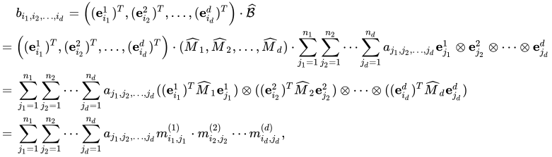
where $\delta _{i,j}$ is the Kronecker delta. Hence, if ${\mathcal {B}}=(M_{1},M_{2},\ldots ,M_{d})\cdot {\mathcal {A}}$ , then

${\begin{aligned}&b_{i_{1},i_{2},\ldots ,i_{d}}=\left((\mathbf {e} _{i_{1}}^{1})^{T},(\mathbf {e} _{i_{2}}^{2})^{T},\ldots ,(\mathbf {e} _{i_{d}}^{d})^{T}\right)\cdot {\widehat {\mathcal {B}}}\\={}&\left((\mathbf {e} _{i_{1}}^{1})^{T},(\mathbf {e} _{i_{2}}^{2})^{T},\ldots ,(\mathbf {e} _{i_{d}}^{d})^{T}\right)\cdot ({\widehat {M}}_{1},{\widehat {M}}_{2},\ldots ,{\widehat {M}}_{d})\cdot \sum _{j_{1}=1}^{n_{1}}\sum _{j_{2}=1}^{n_{2}}\cdots \sum _{j_{d}=1}^{n_{d}}a_{j_{1},j_{2},\ldots ,j_{d}}\mathbf {e} _{j_{1}}^{1}\otimes \mathbf {e} _{j_{2}}^{2}\otimes \cdots \otimes \mathbf {e} _{j_{d}}^{d}\\={}&\sum _{j_{1}=1}^{n_{1}}\sum _{j_{2}=1}^{n_{2}}\cdots \sum _{j_{d}=1}^{n_{d}}a_{j_{1},j_{2},\ldots ,j_{d}}((\mathbf {e} _{i_{1}}^{1})^{T}{\widehat {M}}_{1}\mathbf {e} _{j_{1}}^{1})\otimes ((\mathbf {e} _{i_{2}}^{2})^{T}{\widehat {M}}_{2}\mathbf {e} _{j_{2}}^{2})\otimes \cdots \otimes ((\mathbf {e} _{i_{d}}^{d})^{T}{\widehat {M}}_{d}\mathbf {e} _{j_{d}}^{d})\\={}&\sum _{j_{1}=1}^{n_{1}}\sum _{j_{2}=1}^{n_{2}}\cdots \sum _{j_{d}=1}^{n_{d}}a_{j_{1},j_{2},\ldots ,j_{d}}m_{i_{1},j_{1}}^{(1)}\cdot m_{i_{2},j_{2}}^{(2)}\cdots m_{i_{d},j_{d}}^{(d)},\end{aligned}}$

where the $m_{i,j}^{(k)}$ are the elements of ${\widehat {M}}_{k}$ as defined above.

03Properties

Let ${\mathcal {A}}\in V_{1}\otimes V_{2}\otimes \cdots \otimes V_{d}$ be an order-d tensor over the tensor product of $F$ -vector spaces.

Since a multilinear multiplication is the tensor product of linear maps, we have the following multilinearity property (in the construction of the map):

$A_{1}\otimes \cdots \otimes A_{k-1}\otimes (\alpha A_{k}+\beta B)\otimes A_{k+1}\otimes \cdots \otimes A_{d}=\alpha A_{1}\otimes \cdots \otimes A_{d}+\beta A_{1}\otimes \cdots \otimes A_{k-1}\otimes B\otimes A_{k+1}\otimes \cdots \otimes A_{d}$

Multilinear multiplication is a linear map: $(M_{1},M_{2},\ldots ,M_{d})\cdot (\alpha {\mathcal {A}}+\beta {\mathcal {B}})=\alpha \;(M_{1},M_{2},\ldots ,M_{d})\cdot {\mathcal {A}}+\beta \;(M_{1},M_{2},\ldots ,M_{d})\cdot {\mathcal {B}}$

It follows from the definition that the composition of two multilinear multiplications is also a multilinear multiplication:

$(M_{1},M_{2},\ldots ,M_{d})\cdot \left((K_{1},K_{2},\ldots ,K_{d})\cdot {\mathcal {A}}\right)=(M_{1}\circ K_{1},M_{2}\circ K_{2},\ldots ,M_{d}\circ K_{d})\cdot {\mathcal {A}},$

where $M_{k}:U_{k}\to W_{k}$ and $K_{k}:V_{k}\to U_{k}$ are linear maps.

Observe specifically that multilinear multiplications in different factors commute,

$M_{k}\cdot _{k}\left(M_{\ell }\cdot _{\ell }{\mathcal {A}}\right)=M_{\ell }\cdot _{\ell }\left(M_{k}\cdot _{k}{\mathcal {A}}\right)=M_{k}\cdot _{k}M_{\ell }\cdot _{\ell }{\mathcal {A}},$

if $k\neq \ell .$

04Computation

The factor-k multilinear multiplication $M_{k}\cdot _{k}{\mathcal {A}}$ can be computed in coordinates as follows. Observe first that

${\begin{aligned}M_{k}\cdot _{k}{\mathcal {A}}&=M_{k}\cdot _{k}\sum _{j_{1}=1}^{n_{1}}\sum _{j_{2}=1}^{n_{2}}\cdots \sum _{j_{d}=1}^{n_{d}}a_{j_{1},j_{2},\ldots ,j_{d}}\mathbf {e} _{j_{1}}^{1}\otimes \mathbf {e} _{j_{2}}^{2}\otimes \cdots \otimes \mathbf {e} _{j_{d}}^{d}\\&=\sum _{j_{1}=1}^{n_{1}}\cdots \sum _{j_{k-1}=1}^{n_{k-1}}\sum _{j_{k+1}=1}^{n_{k+1}}\cdots \sum _{j_{d}=1}^{n_{d}}\mathbf {e} _{j_{1}}^{1}\otimes \cdots \otimes \mathbf {e} _{j_{k-1}}^{k-1}\otimes M_{k}\left(\sum _{j_{k}=1}^{n_{k}}a_{j_{1},j_{2},\ldots ,j_{d}}\mathbf {e} _{j_{k}}^{k}\right)\otimes \mathbf {e} _{j_{k+1}}^{k+1}\otimes \cdots \otimes \mathbf {e} _{j_{d}}^{d}.\end{aligned}}$

Next, since

$F^{n_{1}}\otimes F^{n_{2}}\otimes \cdots \otimes F^{n_{d}}\simeq F^{n_{k}}\otimes (F^{n_{1}}\otimes \cdots \otimes F^{n_{k-1}}\otimes F^{n_{k+1}}\otimes \cdots \otimes F^{n_{d}})\simeq F^{n_{k}}\otimes F^{n_{1}\cdots n_{k-1}n_{k+1}\cdots n_{d}},$

there is a bijective map, called the factor-k standard flattening, denoted by $(\cdot )_{(k)}$ , that identifies $M_{k}\cdot _{k}{\mathcal {A}}$ with an element from the latter space, namely

$\left(M_{k}\cdot _{k}{\mathcal {A}}\right)_{(k)}:=\sum _{j_{1}=1}^{n_{1}}\cdots \sum _{j_{k-1}=1}^{n_{k-1}}\sum _{j_{k+1}=1}^{n_{k+1}}\cdots \sum _{j_{d}=1}^{n_{d}}M_{k}\left(\sum _{j_{k}=1}^{n_{k}}a_{j_{1},j_{2},\ldots ,j_{d}}\mathbf {e} _{j_{k}}^{k}\right)\otimes \mathbf {e} _{\mu _{k}(j_{1},\ldots ,j_{k-1},j_{k+1},\ldots ,j_{d})}:=M_{k}{\mathcal {A}}_{(k)},$

where $\mathbf {e} _{j}$ is the jth standard basis vector of $F^{N_{k}}$ , $N_{k}=n_{1}\cdots n_{k-1}n_{k+1}\cdots n_{d}$ , and ${\mathcal {A}}_{(k)}\in F^{n_{k}}\otimes F^{N_{k}}\simeq F^{n_{k}\times N_{k}}$ is the factor-k flattening matrix of ${\mathcal {A}}$ whose columns are the factor-k vectors $[a_{j_{1},\ldots ,j_{k-1},i,j_{k+1},\ldots ,j_{d}}]_{i=1}^{n_{k}}$ in some order, determined by the particular choice of the bijective map

$\mu _{k}:[1,n_{1}]\times \cdots \times [1,n_{k-1}]\times [1,n_{k+1}]\times \cdots \times [1,n_{d}]\to [1,N_{k}].$

In other words, the multilinear multiplication $(M_{1},M_{2},\ldots ,M_{d})\cdot {\mathcal {A}}$ can be computed as a sequence of d factor-k multilinear multiplications, which themselves can be implemented efficiently as classic matrix multiplications.

05Applications

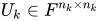
The higher-order singular value decomposition (HOSVD) factorizes a tensor given in coordinates ${\mathcal {A}}\in F^{n_{1}\times n_{2}\times \cdots \times n_{d}}$ as the multilinear multiplication ${\mathcal {A}}=(U_{1},U_{2},\ldots ,U_{d})\cdot {\mathcal {S}}$ , where $U_{k}\in F^{n_{k}\times n_{k}}$ are orthogonal matrices and ${\mathcal {S}}\in F^{n_{1}\times n_{2}\times \cdots \times n_{d}}$ .

Watch videos about Multilinear multiplicationExplainers and documentaries on YouTube (opens in a new tab)

Sources and credits

This article is adapted from the Wikipedia article “Multilinear multiplication”, written by its contributors and licensed under CC BY-SA 4.0. Fathomly has changed the layout, removed citation markers, navigation and maintenance notices, and adjusted punctuation. This adapted version is shared under the same license. For references, see the original article.

Fathomly is not affiliated with or endorsed by the Wikimedia Foundation. Spotted a problem? Tell us.