Encyclopedia

Stokes stream function

Function in fluid dynamics

Wikipedia contributorsAdapted for Fathomly · View authors

2 min read
Source updated January 20, 2026

In fluid dynamics, the Stokes stream function is used to describe the streamlines and flow velocity in a three-dimensional incompressible flow with axisymmetry. A surface with a constant value of the Stokes stream function encloses a streamtube, everywhere tangential to the flow velocity vectors. Further, the volume flux within this streamtube is constant, and all the streamlines of the flow are located on this surface. The velocity field associated with the Stokes stream function is solenoidal, it has zero divergence. This stream function is named in honor of George Gabriel Stokes.

01Cylindrical coordinates

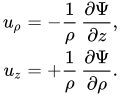
Consider a cylindrical coordinate system ( ρ , φ , z ), with the z, axis the line around which the incompressible flow is axisymmetrical, φ the azimuthal angle and ρ the distance to the z, axis. Then the flow velocity components u_ρ and u_z can be expressed in terms of the Stokes stream function $\Psi$ by:

${\begin{aligned}u_{\rho }&=-{\frac {1}{\rho }}\,{\frac {\partial \Psi }{\partial z}},\\u_{z}&=+{\frac {1}{\rho }}\,{\frac {\partial \Psi }{\partial \rho }}.\end{aligned}}$

The azimuthal velocity component u_φ does not depend on the stream function. Due to the axisymmetry, all three velocity components ( u_ρ , u_φ , u_z ) only depend on ρ and z and not on the azimuth φ.

The volume flux, through the surface bounded by a constant value ψ of the Stokes stream function, is equal to 2π ψ.

02Spherical coordinates

In spherical coordinates ( r , θ , φ ), r is the radial distance from the origin, θ is the zenith angle and φ is the azimuthal angle. In axisymmetric flow, with θ = 0 the rotational symmetry axis, the quantities describing the flow are again independent of the azimuth φ. The flow velocity components u_r and u_θ are related to the Stokes stream function $\Psi$ through:

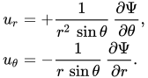
${\begin{aligned}u_{r}&=+{\frac {1}{r^{2}\,\sin \theta }}\,{\frac {\partial \Psi }{\partial \theta }},\\u_{\theta }&=-{\frac {1}{r\,\sin \theta }}\,{\frac {\partial \Psi }{\partial r}}.\end{aligned}}$

Again, the azimuthal velocity component u_φ is not a function of the Stokes stream function ψ. The volume flux through a stream tube, bounded by a surface of constant ψ, equals 2π ψ, as before.

Vorticity

The vorticity is defined as:

${\boldsymbol {\omega }}=\nabla \times {\boldsymbol {u}}=\nabla \times \nabla \times {\boldsymbol {\psi }}$ , where ${\boldsymbol {\psi }}={\frac {\Psi }{r\sin \theta }}{\boldsymbol {\hat {\phi }}},$

with ${\boldsymbol {\hat {\phi }}}$ the unit vector in the $\phi \,$ , direction.

Derivation of vorticity ${\boldsymbol {\omega }}$ using a Stokes stream function
Consider the vorticity as defined by ${\boldsymbol {\omega }}=\nabla \times {\boldsymbol {u}}.$ From the definition of the curl in spherical coordinates: ${\begin{aligned}\omega _{r}&={1 \over r\sin \theta }\left({\partial \over \partial \theta }\left(u_{\phi }\sin \theta \right)-{\partial u_{\theta } \over \partial \phi }\right){\boldsymbol {\hat {r}}},\\\omega _{\theta }&={1 \over r}\left({1 \over \sin \theta }{\partial u_{r} \over \partial \phi }-{\partial \over \partial r}\left(ru_{\phi }\right)\right){\boldsymbol {\hat {\theta }}},\\\omega _{\phi }&={1 \over r}\left({\partial \over \partial r}\left(ru_{\theta }\right)-{\partial u_{r} \over \partial \theta }\right){\boldsymbol {\hat {\phi }}}.\end{aligned}}$ First notice that the $r$ and $\theta$ components are equal to 0. Secondly substitute $u_{r}$ and $u_{\theta }$ into $\omega _{\phi }.$ The result is: ${\begin{aligned}\omega _{r}&=0,\\\omega _{\theta }&=0,\\\omega _{\phi }&={1 \over r}\left({\partial \over \partial r}\left(r\left(-{\frac {1}{r\sin \theta }}{\frac {\partial \Psi }{\partial r}}\right)\right)-{\partial \over \partial \theta }\left({\frac {1}{r^{2}\sin \theta }}{\frac {\partial \Psi }{\partial \theta }}\right)\right).\end{aligned}}$ Next the following algebra is performed: ${\begin{aligned}\omega _{\phi }&={1 \over r}\left(-{\frac {1}{\sin \theta }}\left({\partial \over \partial r}\left({\frac {\partial \Psi }{\partial r}}\right)\right)-{\frac {1}{r^{2}}}{\partial \over \partial \theta }\left({\frac {1}{\sin \theta }}{\frac {\partial \Psi }{\partial \theta }}\right)\right)\\&={1 \over r}\left(-{\frac {1}{\sin \theta }}\left({\frac {\partial ^{2}\Psi }{\partial r^{2}}}\right)-{\frac {\sin \theta }{r^{2}\sin \theta }}{\partial \over \partial \theta }\left({\frac {1}{\sin \theta }}{\frac {\partial \Psi }{\partial \theta }}\right)\right)\\&=-{\frac {1}{r\sin \theta }}\left({\frac {\partial ^{2}\Psi }{\partial r^{2}}}+{\frac {\sin \theta }{r^{2}}}{\partial \over \partial \theta }\left({\frac {1}{\sin \theta }}{\frac {\partial \Psi }{\partial \theta }}\right)\right).\end{aligned}}$

Derivation of vorticity ${\boldsymbol {\omega }}$ using a Stokes stream function

Consider the vorticity as defined by

${\boldsymbol {\omega }}=\nabla \times {\boldsymbol {u}}.$

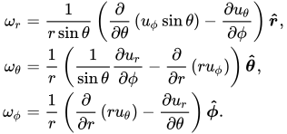
From the definition of the curl in spherical coordinates:

${\begin{aligned}\omega _{r}&={1 \over r\sin \theta }\left({\partial \over \partial \theta }\left(u_{\phi }\sin \theta \right)-{\partial u_{\theta } \over \partial \phi }\right){\boldsymbol {\hat {r}}},\\\omega _{\theta }&={1 \over r}\left({1 \over \sin \theta }{\partial u_{r} \over \partial \phi }-{\partial \over \partial r}\left(ru_{\phi }\right)\right){\boldsymbol {\hat {\theta }}},\\\omega _{\phi }&={1 \over r}\left({\partial \over \partial r}\left(ru_{\theta }\right)-{\partial u_{r} \over \partial \theta }\right){\boldsymbol {\hat {\phi }}}.\end{aligned}}$

First notice that the $r$ and $\theta$ components are equal to 0. Secondly substitute $u_{r}$ and $u_{\theta }$ into $\omega _{\phi }.$ The result is:

${\begin{aligned}\omega _{r}&=0,\\\omega _{\theta }&=0,\\\omega _{\phi }&={1 \over r}\left({\partial \over \partial r}\left(r\left(-{\frac {1}{r\sin \theta }}{\frac {\partial \Psi }{\partial r}}\right)\right)-{\partial \over \partial \theta }\left({\frac {1}{r^{2}\sin \theta }}{\frac {\partial \Psi }{\partial \theta }}\right)\right).\end{aligned}}$

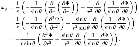
Next the following algebra is performed:

${\begin{aligned}\omega _{\phi }&={1 \over r}\left(-{\frac {1}{\sin \theta }}\left({\partial \over \partial r}\left({\frac {\partial \Psi }{\partial r}}\right)\right)-{\frac {1}{r^{2}}}{\partial \over \partial \theta }\left({\frac {1}{\sin \theta }}{\frac {\partial \Psi }{\partial \theta }}\right)\right)\\&={1 \over r}\left(-{\frac {1}{\sin \theta }}\left({\frac {\partial ^{2}\Psi }{\partial r^{2}}}\right)-{\frac {\sin \theta }{r^{2}\sin \theta }}{\partial \over \partial \theta }\left({\frac {1}{\sin \theta }}{\frac {\partial \Psi }{\partial \theta }}\right)\right)\\&=-{\frac {1}{r\sin \theta }}\left({\frac {\partial ^{2}\Psi }{\partial r^{2}}}+{\frac {\sin \theta }{r^{2}}}{\partial \over \partial \theta }\left({\frac {1}{\sin \theta }}{\frac {\partial \Psi }{\partial \theta }}\right)\right).\end{aligned}}$

As a result, from the calculation the vorticity vector is found to be equal to:

${\boldsymbol {\omega }}={\begin{pmatrix}0\\[1ex]0\\[1ex]\displaystyle -{\frac {1}{r\sin \theta }}\left({\frac {\partial ^{2}\Psi }{\partial r^{2}}}+{\frac {\sin \theta }{r^{2}}}{\partial \over \partial \theta }\left({\frac {1}{\sin \theta }}{\frac {\partial \Psi }{\partial \theta }}\right)\right)\end{pmatrix}}.$

Comparison with cylindrical

The cylindrical and spherical coordinate systems are related through

$z=r\,\cos \theta \,$ and $\rho =r\,\sin \theta .\,$

03Alternative definition with opposite sign

As explained in the general stream function article, definitions using an opposite sign convention, for the relationship between the Stokes stream function and flow velocity, are also in use.

04Zero divergence

In cylindrical coordinates, the divergence of the velocity field u becomes:

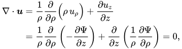
${\begin{aligned}\nabla \cdot {\boldsymbol {u}}&={\frac {1}{\rho }}{\frac {\partial }{\partial \rho }}{\Bigl (}\rho \,u_{\rho }{\Bigr )}+{\frac {\partial u_{z}}{\partial z}}\\&={\frac {1}{\rho }}{\frac {\partial }{\partial \rho }}\left(-{\frac {\partial \Psi }{\partial z}}\right)+{\frac {\partial }{\partial z}}\left({\frac {1}{\rho }}{\frac {\partial \Psi }{\partial \rho }}\right)=0,\end{aligned}}$

as expected for an incompressible flow.

And in spherical coordinates:

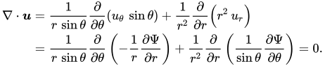
${\begin{aligned}\nabla \cdot {\boldsymbol {u}}&={\frac {1}{r\,\sin \theta }}{\frac {\partial }{\partial \theta }}(u_{\theta }\,\sin \theta )+{\frac {1}{r^{2}}}{\frac {\partial }{\partial r}}{\Bigl (}r^{2}\,u_{r}{\Bigr )}\\&={\frac {1}{r\,\sin \theta }}{\frac {\partial }{\partial \theta }}\left(-{\frac {1}{r}}{\frac {\partial \Psi }{\partial r}}\right)+{\frac {1}{r^{2}}}{\frac {\partial }{\partial r}}\left({\frac {1}{\sin \theta }}{\frac {\partial \Psi }{\partial \theta }}\right)=0.\end{aligned}}$

05Streamlines as curves of constant stream function

From calculus it is known that the gradient vector $\nabla \Psi$ is normal to the curve $\Psi =C$ (see e.g. Level set#Level sets versus the gradient). If it is shown that everywhere ${\boldsymbol {u}}\cdot \nabla \Psi =0,$ using the formula for ${\boldsymbol {u}}$ in terms of $\Psi ,$ then this proves that level curves of $\Psi$ are streamlines.

Cylindrical coordinates

In cylindrical coordinates,

$\nabla \Psi ={\partial \Psi \over \partial \rho }{\boldsymbol {e}}_{\rho }+{\partial \Psi \over \partial z}{\boldsymbol {e}}_{z}$ .

and

${\boldsymbol {u}}=u_{\rho }{\boldsymbol {e}}_{\rho }+u_{z}{\boldsymbol {e}}_{z}=-{1 \over \rho }{\partial \Psi \over \partial z}{\boldsymbol {e}}_{\rho }+{1 \over \rho }{\partial \Psi \over \partial \rho }{\boldsymbol {e}}_{z}.$

So that

$\nabla \Psi \cdot {\boldsymbol {u}}={\partial \Psi \over \partial \rho }(-{1 \over \rho }{\partial \Psi \over \partial z})+{\partial \Psi \over \partial z}{1 \over \rho }{\partial \Psi \over \partial \rho }=0.$

Spherical coordinates

And in spherical coordinates

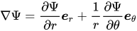
$\nabla \Psi ={\partial \Psi \over \partial r}{\boldsymbol {e}}_{r}+{1 \over r}{\partial \Psi \over \partial \theta }{\boldsymbol {e}}_{\theta }$

and

${\boldsymbol {u}}=u_{r}{\boldsymbol {e}}_{r}+u_{\theta }{\boldsymbol {e}}_{\theta }={1 \over r^{2}\sin \theta }{\partial \Psi \over \partial \theta }{\boldsymbol {e}}_{r}-{1 \over r\sin \theta }{\partial \Psi \over \partial r}{\boldsymbol {e}}_{\theta }.$

So that

$\nabla \Psi \cdot {\boldsymbol {u}}={\partial \Psi \over \partial r}\cdot {1 \over r^{2}\sin \theta }{\partial \Psi \over \partial \theta }+{1 \over r}{\partial \Psi \over \partial \theta }\cdot {\Big (}-{1 \over r\sin \theta }{\partial \Psi \over \partial r}{\Big )}=0.$

Watch videos about Stokes stream functionExplainers and documentaries on YouTube (opens in a new tab)

Sources and credits

This article is adapted from the Wikipedia article “Stokes stream function”, written by its contributors and licensed under CC BY-SA 4.0. Fathomly has changed the layout, removed citation markers, navigation and maintenance notices, and adjusted punctuation. This adapted version is shared under the same license. For references, see the original article.

Images, from Wikimedia Commons:

Stokes sphere.svg by Kraaiennest, CC BY-SA 3.0
Cylindrical with grid.svg by Andeggs, CC BY-SA 4.0
Spherical with grid.svg by Andeggs, CC BY-SA 4.0

Fathomly is not affiliated with or endorsed by the Wikimedia Foundation. Spotted a problem? Tell us.