Encyclopedia

Spin glass

Disordered magnetic state

Wikipedia contributorsAdapted for Fathomly · View authors

13 min read
Source updated August 27, 2026

In condensed matter physics, a spin glass is a magnetic state characterized by randomness, despite cooperative behavior in freezing of spins at a temperature called the "freezing temperature," T_f. In ferromagnetic solids, component atoms' magnetic spins all align in the same direction. When contrasted with a ferromagnet, a spin glass is defined as a "disordered" magnetic state in which spins are aligned and coupled without a regular pattern. A spin glass should not be confused with a "spin-on glass." The latter is a thin film which is applied via spin coating, and is usually based on SiO₂.

The term "glass" comes from an analogy between the magnetic disorder in a spin glass and the positional disorder of a conventional, chemical glass (e.g., a window glass). In any amorphous solid, such as window glass, the atomic bond structure is highly irregular; in contrast, a crystal has a uniform pattern of atomic bonds. In ferromagnetic solids, magnetic spins all align in the same direction; this is analogous to a crystal's lattice-based structure.

The individual atomic bonds in a spin glass are a mixture of roughly equal numbers of ferromagnetic bonds (where neighbors have the same orientation) and antiferromagnetic bonds (where neighbors have exactly the opposite orientation, where north and south poles are flipped 180 degrees). These patterns of aligned and misaligned atomic magnets create what are known as frustrated interactions , distortions in the geometry of atomic bonds compared to what would be seen in a regular, fully aligned solid. They may also create situations where more than one geometric arrangement of atoms is stable.

There are two main aspects of spin glass. On the physical side, spin glasses are real materials with distinctive properties, a review of which was published in 1982. On the mathematical side, models from statistical mechanics inform the study of both real spin glasses and analogous systems (e.g., human social systems).

Spin glasses and the complex internal structures that arise within them are termed "metastable" because they are "stuck" in stable configurations other than the lowest-energy configuration (which would be aligned and ferromagnetic). While difficult, the study of spin glasses has yielded valuable results in fields outside of physics, including chemistry, computer science and neural networks, pure mathematics, complex systems science, and even sociology.

01Magnetic behavior

The key methods of determining whether a material is a spin glass are rooted in its magnetic behavior. Because of the underlying disordered structure of the magnetic moments, a spin glass is expected to exhibit a unique combination of features. A list of necessary criteria is proposed by Mydosh in a review paper:

The ac susceptibility $\chi _{\mathrm {ac} }=\chi '+i\chi ''={\frac {\partial M}{\partial B_{ac}}}$ is the response of the spin glass to an alternating magnetic field. It consists of an (reactive) in-phase component $\chi '$ and an (absorptive) out-of-phase component $\chi ''$ . The expectation for a spin glass is that $\chi ''(T)$ peaks sharply at the freezing temperature $T_{f}$ . It is, furthermore expected that the freezing temperature is only weakly dependent on the excitation frequency. An explanation for this is that during the freezing process, the fluctuations lead to a slowing down of the spin dynamics and thus a higher absorption $\chi ''$ .
The temperature dependent magnetization $M(T)$ in the frozen state must depend on the magnetic history: A pronounced splitting between the magnetization in heating must occur where a constant $M$ is expected up to $T_{f}$ when the sample was cooled across the transition in a magnetic field (so called field cooled FC). This is opposed to a field-free cooling and application of the magnetic field only in the frozen state (zero-field cooling ZFC). Underlying this is that the glass is frozen into a (partially) magnetized state in a FC protocol.
The magnetic specific heat $c_{m}$ shows a broad, field-dependent maximum at $T_{f}$ , whereas it is sharp at the transition to an ordered state (like a ferro- or antiferromagnet).
Because spin glasses are based on disorder, there is a decay of the magnetized state, it ages. This means that a zero-field cooled magnetized state will decay back into an unmagnetized one. There will be a maximum in the quantity $S(t)=(1/H){\frac {\partial M}{\partial \ln t}}$ .

Above the spin glass transition temperature, T_c, the spin glass exhibits typical magnetic behaviour (such as paramagnetism).

If a magnetic field is applied as the sample is cooled to the transition temperature, magnetization of the sample increases as described by the Curie law.

Surprisingly, the sum of the two complicated functions of time (the zero-field-cooled and remanent magnetizations) is a constant, namely the field-cooled value, and thus both share identical functional forms with time, at least in the limit of very small external fields.

02Edwards-Anderson model

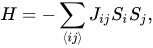
The Edwards-Anderson model is similar to the Ising model, in which spins are arranged on a $d$ -dimensional lattice with only nearest neighbor interactions. Critical temperatures can be solved for exactly and a glassy phase is observed to exist at low temperatures. The Hamiltonian for this spin system is given by

$H=-\sum _{\langle ij\rangle }J_{ij}S_{i}S_{j},$

where $S_{i}$ refers to the Pauli spin matrix for the spin-half particle at lattice point $i$ and the sum over $\langle ij\rangle$ includes all nearest-neighbor lattice points $i$ and $j$ . The variables $J_{ij}$ characterize the magnetic interactions between neighboring spins and are called bond or link variables. The interaction is antiferromagnetic for negative $J_{ij}$ and ferromagnetic for positive $J_{ij}$ .

In order to determine the partition function for this system, one needs to average the free energy $f\left[J_{ij}\right]=-{\frac {1}{\beta }}\ln {\mathcal {Z}}\left[J_{ij}\right]$ where ${\mathcal {Z}}\left[J_{ij}\right]=\operatorname {Tr} _{S}\left(e^{-\beta H}\right)$ , over all possible values of $J_{ij}$ . The distribution of values of $J_{ij}$ is taken to be a Gaussian with a mean $J_{0}$ and a variance $J^{2}$ :

$P(J_{ij})={\sqrt {\frac {N}{2\pi J^{2}}}}\exp \left\{-{\frac {N}{2J^{2}}}\left(J_{ij}-{\frac {J_{0}}{N}}\right)^{2}\right\}.$

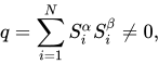
For the +J and -J random-bond Ising model, in which nearest-neighbor couplings take the values +J and -J with probabilities p and 1 - p, the Nishimori line is the locus in the temperature-disorder phase diagram satisfying $\exp(-2\beta J)=(1-p)/p$ . On this line, gauge transformations give exact results such as the internal energy, making it one of the few exactly controlled cases of finite-dimensional spin-glass models. In information-processing applications, Nishimori used related spin-glass methods to show that, for certain error-correcting code ensembles, the decoding error can be minimized at a finite decoding temperature matched to the channel noise. Iba later discussed the Nishimori line from the viewpoint of Bayesian statistics.

Solving for the free energy using the replica method, below a certain temperature, a new magnetic phase called the spin glass phase (or glassy phase) of the system is found to exist which is characterized by a vanishing magnetization $m=0$ along with a non-vanishing value of the two point correlation function between spins at the same lattice point but at two different replicas:

$q=\sum _{i=1}^{N}S_{i}^{\alpha }S_{i}^{\beta }\neq 0,$

where $\alpha ,\beta$ are replica indices. The order parameter for the ferromagnetic to spin glass phase transition is therefore $q$ , and that for paramagnetic to spin glass is again $q$ . Hence the new set of order parameters describing the three magnetic phases consists of both $m$ and $q$ .

Under the assumption of replica symmetry, the mean-field free energy is given by the expression:

${\begin{aligned}\beta f={}-{\frac {\beta ^{2}J^{2}}{4}}(1-q)^{2}+{\frac {\beta J_{0}m^{2}}{2}}-\int \exp \left(-{\frac {z^{2}}{2}}\right)\log \left(2\cosh \left(\beta Jz+\beta J_{0}m\right)\right)\,\mathrm {d} z.\end{aligned}}$

03Sherrington-Kirkpatrick model

In addition to unusual experimental properties, spin glasses are the subject of extensive theoretical and computational investigations. A substantial part of early theoretical work on spin glasses dealt with a form of mean-field theory based on a set of replicas of the partition function of the system.

An important, exactly solvable model of a spin glass was introduced by David Sherrington and Scott Kirkpatrick in 1975. It is an Ising model with long range frustrated ferro- as well as antiferromagnetic couplings. It corresponds to a mean-field approximation of spin glasses describing the slow dynamics of the magnetization and the complex non-ergodic equilibrium state.

Unlike the Edwards-Anderson (EA) model, the range of each spin-spin interaction can be arbitrarily large (not restricted to neighboring sites). Any two spins can be linked with a ferromagnetic or an antiferromagnetic bond; the distribution of these bonds is the same as in the EA model. The SK Hamiltonian is

$H=-{\frac {1}{\sqrt {N}}}\sum _{i<j}J_{ij}S_{i}S_{j},$

where $J_{ij},S_{i},S_{j}$ have same meanings as in the EA model. The equilibrium solution of the model, after initial attempts by Sherrington, Kirkpatrick and others, was found by Giorgio Parisi in 1979 using the replica method. The subsequent work interpreting the Parisi solution, by M. Mezard, G. Parisi, M.A. Virasoro and many others, revealed the complex nature of glassy, low-temperature phases, characterized by ergodicity breaking, ultrametricity and non-selfaverageness. Further developments led to the creation of the cavity method, which allowed study of the low-temperature phase without replicas. A rigorous proof of the Parisi solution has been provided in the work of Francesco Guerra and Michel Talagrand.

Phase diagram

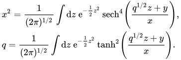
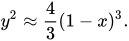
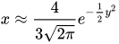
When there is a uniform external magnetic field of magnitude $M$ , the energy function becomes $H=-{\frac {1}{\sqrt {N}}}\sum _{i<j}J_{ij}S_{i}S_{j}-M\sum _{i}S_{i}$ Let all couplings $J_{ij}$ are IID samples from the gaussian distribution of mean 0 and variance $J^{2}$ . In 1979, J.R.L. de Almeida and David Thouless found that, as in the case of the Ising model, the mean-field solution to the SK model becomes unstable when under low-temperature, low-magnetic field state.

The stability region on the phase diagram of the SK model is determined by two dimensionless parameters 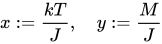$x:={\frac {kT}{J}},\quad y:={\frac {M}{J}}$ . Its phase diagram has two parts, divided by the de Almeida-Thouless curve, The curve is the solution set to the equations ${\begin{aligned}&x^{2}={\frac {1}{(2\pi )^{1/2}}}\int \mathrm {d} z\;\mathrm {e} ^{-{\frac {1}{2}}z^{2}}\operatorname {sech} ^{4}\left({\frac {q^{1/2}z+y}{x}}\right),\\&q={\frac {1}{(2\pi )^{1/2}}}\int \mathrm {d} z\;\mathrm {e} ^{-{\frac {1}{2}}z^{2}}\tanh ^{2}\left({\frac {q^{1/2}z+y}{x}}\right).\end{aligned}}$ The phase transition occurs at $x=1$ . Just below it, we have $y^{2}\approx {\frac {4}{3}}(1-x)^{3}.$ At low temperature, high magnetic field limit, the line is $x\approx {\frac {4}{3{\sqrt {2\pi }}}}e^{-{\frac {1}{2}}y^{2}}$

04Infinite-range model

This is also called the "p-spin model". The infinite-range model is a generalization of the Sherrington-Kirkpatrick model where we not only consider two-spin interactions but $p$ -spin interactions, where $p\leq N$ and $N$ is the total number of spins. Unlike the Edwards-Anderson model, but similar to the SK model, the interaction range is infinite. The Hamiltonian for this model is described by:

$H=-\sum _{i_{1}<i_{2}<\cdots <i_{p}}J_{i_{1}\dots i_{p}}S_{i_{1}}\cdots S_{i_{p}}$

where $J_{i_{1}\dots i_{p}},S_{i_{1}},\dots ,S_{i_{p}}$ have similar meanings as in the EA model. The $p\to \infty$ limit of this model is known as the random energy model. In this limit, the probability of the spin glass existing in a particular state depends only on the energy of that state and not on the individual spin configurations in it. A Gaussian distribution of magnetic bonds across the lattice is assumed usually to solve this model. Any other distribution is expected to give the same result, as a consequence of the central limit theorem. The Gaussian distribution function, with mean ${\frac {J_{0}}{N}}$ and variance ${\frac {J^{2}}{N}}$ , is given as:

$P\left(J_{i_{1}\cdots i_{p}}\right)={\sqrt {\frac {N^{p-1}}{J^{2}\pi p!}}}\exp \left\{-{\frac {N^{p-1}}{J^{2}p!}}\left(J_{i_{1}\cdots i_{p}}-{\frac {J_{0}p!}{2N^{p-1}}}\right)\right\}$

The order parameters for this system are given by the magnetization $m$ and the two point spin correlation between spins at the same site $q$ , in two different replicas, which are the same as for the SK model. This infinite range model can be solved explicitly for the free energy in terms of $m$ and $q$ , under the assumption of replica symmetry as well as 1-Replica Symmetry Breaking.

${\begin{aligned}\beta f={}&{\frac {1}{4}}\beta ^{2}J^{2}q^{p}-{\frac {1}{2}}p\beta ^{2}J^{2}q^{p}-{\frac {1}{4}}\beta ^{2}J^{2}+{\frac {1}{2}}\beta J_{0}pm^{p}+{\frac {1}{4{\sqrt {2\pi }}}}p\beta ^{2}J^{2}q^{p-1}+{}\\&\int \exp \left(-{\frac {1}{2}}z^{2}\right)\log \left(2\cosh \left(\beta Jz{\sqrt {{\frac {1}{2}}pq^{p-1}}}+{\frac {1}{2}}\beta J_{0}pm^{p-1}\right)\right)\,\mathrm {d} z\end{aligned}}$

05Non-ergodic behavior and applications

A thermodynamic system is ergodic when, given any (equilibrium) instance of the system, it eventually visits every other possible (equilibrium) state (of the same energy). One characteristic of spin glass systems is that, below the freezing temperature $T_{\text{f}}$ , instances are trapped in a "non-ergodic" set of states: the system may fluctuate between several states, but cannot transition to other states of equivalent energy. Intuitively, one can say that the system cannot escape from deep minima of the hierarchically disordered energy landscape; the distances between minima are given by an ultrametric, with tall energy barriers between minima. The participation ratio counts the number of states that are accessible from a given instance, that is, the number of states that participate in the ground state. The ergodic aspect of spin glass was instrumental in the awarding of half the 2021 Nobel Prize in Physics to Giorgio Parisi.

For physical systems, such as dilute manganese in copper, the freezing temperature is typically as low as 30 kelvins (−240 °C), and so the spin-glass magnetism appears to be practically without applications in daily life. The non-ergodic states and rugged energy landscapes are, however, quite useful in understanding the behavior of certain neural networks, including Hopfield networks, as well as many problems in computer science optimization and genetics.

06Spin-glass without structural disorder

Elemental crystalline neodymium is paramagnetic at room temperature and becomes an antiferromagnet with incommensurate order upon cooling below 19.9 K. Below this transition temperature it exhibits a complex set of magnetic phases that have long spin relaxation times and spin-glass behavior that does not rely on structural disorder.

07History

A detailed account of the history of spin glasses from the early 1960s to the late 1980s can be found in a series of popular articles by Philip W. Anderson in Physics Today.

Discovery

In 1930s, material scientists discovered the Kondo effect, where the resistivity of nominally pure gold reaches a minimum at 10 K, and similarly for nominally pure Cu at 2 K. It was later understood that the Kondo effect occurs when a nonmagnetic metal contains a very small fraction of magnetic atoms (i.e., at high dilution).

Unusual behavior was observed in iron-in-gold alloy (AuFe) and manganese-in-copper alloy (CuMn) at around 1 to 10 atom percent. Cannella and Mydosh observed in 1972 that AuFe had an unexpected cusplike peak in the a.c. susceptibility at a well defined temperature, which would later be termed spin glass freezing temperature.

It was also called "mictomagnet" (micto- is Greek for "mixed"). The term arose from the observation that these materials often contain a mix of ferromagnetic ( $J>0$ ) and antiferromagnetic ( $J<0$ ) interactions, leading to their disordered magnetic structure. This term fell out of favor as the theoretical understanding of spin glasses evolved, recognizing that the magnetic frustration arises not just from a simple mixture of ferro- and antiferromagnetic interactions, but from their randomness and frustration in the system.

Sherrington-Kirkpatrick model

Sherrington and Kirkpatrick proposed the SK model in 1975, and solved it by the replica method. They discovered that at low temperatures, its entropy becomes negative, which they thought was because the replica method is a heuristic method that does not apply at low temperatures.

It was then discovered that the replica method was correct, but the problem lies in that the low-temperature broken symmetry in the SK model cannot be purely characterized by the Edwards-Anderson order parameter. Instead, further order parameters are necessary, which leads to replica breaking ansatz of Giorgio Parisi. At the full replica breaking ansatz, infinitely many order parameters are required to characterize a stable solution.

08Applications

The formalism of replica mean-field theory has also been applied in the study of neural networks, where it has enabled calculations of properties such as the storage capacity of simple neural network architectures without requiring a training algorithm (such as backpropagation) to be designed or implemented.

More realistic spin glass models with short range frustrated interactions and disorder, like the Gaussian model where the couplings between neighboring spins follow a Gaussian distribution, have been studied extensively as well, especially using Monte Carlo simulations. These models display spin glass phases bordered by sharp phase transitions.

Besides its relevance in condensed matter physics, spin glass theory has acquired a strongly interdisciplinary character, with applications to neural network theory, computer science, theoretical biology, econophysics etc.

Spin glass models were adapted to the folding funnel model of protein folding.

09Literature

Expositions

Stein, Daniel L.; Newman, Charles M. (2013). Spin glasses and complexity. Primers in complex systems. Princeton: Princeton University Press. ISBN 978-0-691-14733-8. Popular exposition, with a minimal amount of mathematics.
Montanari, Andrea; Sen, Subhabrata (2024-01-09). "A Friendly Tutorial on Mean-Field Spin Glass Techniques for Non-Physicists". Foundations and Trends in Machine Learning. 17 (1): 1, 173. arXiv:2204.02909. doi:10.1561/2200000105. ISSN 1935-8237. A practical tutorial introduction.
Mézard, Marc; Montanari, Andrea (2009). Information, Physics, and Computation. Oxford, U.K.: Oxford University Press. ISBN 978-0-19-857083-7. OCLC 234430714. 1st 15 chapters of 2008 draft version, available at www.stat.ucla.edu Textbook that focuses on the cavity method and the applications to computer science, especially constraint satisfaction problems.
Nishimori, Hidetoshi (2001). Statistical physics of spin glasses and information processing: an introduction. International series of monographs on physics. Oxford; New York: Oxford University Press. ISBN 978-0-19-850940-0. OCLC 47063323. Introduction focused on computer science applications, including neural networks.
Mydosh, J. A. (1993). Spin glasses: an experimental introduction. London; Washington, DC: Taylor & Francis. ISBN 978-0-7484-0038-6. Focuses on the experimentally measurable properties of spin glasses (such as copper-manganese alloy).
Fischer, K. H.; Hertz, John (1991). Spin glasses. Cambridge studies in magnetism. Cambridge; New York, NY, USA: Cambridge University Press. ISBN 978-0-521-34296-4. Covers mean field theory, experimental data, and numerical simulations.
Mezard, Marc; Parisi, Giorgio; Virasoro, Miguel Angel (1987), Spin glass theory and beyond, Singapore: World Scientific, ISBN 978-9971-5-0115-0. Early exposition containing the pre-1990 breakthroughs, such as the replica trick.
De Dominicis, Cirano; Giardina, Irene (2006). Random fields and spin glasses: a field theory approach. Cambridge, UK; New York: Cambridge University Press. ISBN 978-0-521-84783-4. OCLC 70764844. Approach via statistical field theory.
Talagrand, Michel (2010). Mean field models for spin glasses. 1: Basic examples. Ergebnisse der Mathematik und ihrer Grenzgebiete (Softcover repr. of the harcover 1st ed. 2010 ed.). Berlin Heidelberg: Springer. ISBN 978-3-642-26598-3. and Talagrand, Michel (2011). Mean field models for spin glasses. Ergebnisse der Mathematik und ihrer Grenzgebiete. 3. Folge = A series of modern surveys in mathematics. Heidelberg; New York: Springer. ISBN 978-3-642-15201-6. OCLC 733249730.. Compendium of rigorously provable results.

Primary sources

Edwards, S.F.; Anderson, P.W. (1975), "Theory of spin glasses", Journal of Physics F: Metal Physics, 5 (5): 965, 974, Bibcode:1975JPhF....5..965E, doi:10.1088/0305-4608/5/5/017. ShieldSquare Captcha
Sherrington, David; Kirkpatrick, Scott (1975), "Solvable model of a spin-glass", Physical Review Letters, 35 (26): 1792, 1796, Bibcode:1975PhRvL..35.1792S, doi:10.1103/PhysRevLett.35.1792. Papercore Summary http://papercore.org/Sherrington1975^{[link removed]}
Nordblad, P.; Lundgren, L.; Sandlund, L. (1986), "A link between the relaxation of the zero field cooled and the thermoremanent magnetizations in spin glasses", Journal of Magnetism and Magnetic Materials, 54: 185, 186, Bibcode:1986JMMM...54..185N, doi:10.1016/0304-8853(86)90543-3.
Binder, K.; Young, A. P. (1986), "Spin glasses: Experimental facts, theoretical concepts, and open questions", Reviews of Modern Physics, 58 (4): 801, 976, Bibcode:1986RvMP...58..801B, doi:10.1103/RevModPhys.58.801.
Bryngelson, Joseph D.; Wolynes, Peter G. (1987), "Spin glasses and the statistical mechanics of protein folding", Proceedings of the National Academy of Sciences, 84 (21): 7524, 7528, Bibcode:1987PNAS...84.7524B, doi:10.1073/pnas.84.21.7524, PMC 299331, PMID 3478708....
Parisi, G. (1980), "The order parameter for spin glasses: a function on the interval 0-1" (PDF), J. Phys. A: Math. Gen., 13 (3): 1101, 1112, Bibcode:1980JPhA...13.1101P, doi:10.1088/0305-4470/13/3/042, archived from the original (PDF) on September 22, 2017 Papercore Summary http://papercore.org/Parisi1980^{[link removed]}.
Talagrand, Michel (2000), "Replica symmetry breaking and exponential inequalities for the Sherrington-Kirkpatrick model", Annals of Probability, 28 (3): 1018, 1062, doi:10.1214/aop/1019160325, JSTOR 2652978.
Guerra, F.; Toninelli, F. L. (2002), "The thermodynamic limit in mean field spin glass models", Communications in Mathematical Physics, 230 (1): 71, 79, arXiv:cond-mat/0204280, Bibcode:2002CMaPh.230...71G, doi:10.1007/s00220-002-0699-y, S2CID 16833848

Watch videos about Spin glassExplainers and documentaries on YouTube (opens in a new tab)

Sources and credits

This article is adapted from the Wikipedia article “Spin glass”, written by its contributors and licensed under CC BY-SA 4.0. Fathomly has changed the layout, removed citation markers, navigation and maintenance notices, and adjusted punctuation. This adapted version is shared under the same license. For references, see the original article.

Images, from Wikimedia Commons:

Spin glass by Zureks.svg by Zureks, CC0
De Almeida-Thouless line.svg by Cosmia Nebula, CC BY-SA 4.0

Fathomly is not affiliated with or endorsed by the Wikimedia Foundation. Spotted a problem? Tell us.