Spectral element method

The spectral method expands the solution in trigonometric series, a chief advantage being that the resulting method is of a very high order. This approach relies on the fact that trigonometric polynomials are an orthonormal basis for . The spectral element method chooses instead a high degree piecewise polynomial basis functions, also achieving a very high order of accuracy. Such polynomials are usually orthogonal Chebyshev polynomials or very high order Lagrange polynomials over non-uniformly spaced nodes. In SEM computational error decreases exponentially as the order of approximating polynomial increases, therefore a fast convergence of solution to the exact solution is realized with fewer degrees of freedom of the structure in comparison with FEM. In structural health monitoring, FEM can be used for detecting large flaws in a structure, but as the size of the flaw is reduced there is a need to use a high-frequency wave. In order to simulate the propagation of a high-frequency wave, the FEM mesh required is very fine resulting in increased computational time. On the other hand, SEM provides good accuracy with fewer degrees of freedom. Non-uniformity of nodes helps to make the mass matrix diagonal, which saves time and memory and is also useful for adopting a central difference method (CDM). The disadvantages of SEM include difficulty in modeling complex geometry, compared to the flexibility of FEM.

Although the method can be applied with a modal piecewise orthogonal polynomial basis, it is most often implemented with a nodal tensor product Lagrange basis. The method gains its efficiency by placing the nodal points at the Legendre-Gauss-Lobatto (LGL) points and performing the Galerkin method integrations with a reduced Gauss-Lobatto quadrature using the same nodes. With this combination, simplifications result such that mass lumping occurs at all nodes and a collocation procedure results at interior points.

The most popular applications of the method are in computational fluid dynamics and modeling seismic wave propagation.

The classic analysis of Galerkin methods and Céa's lemma holds here and it can be shown that, if is the solution of the weak equation, is the approximate solution and :

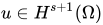
where is related to the discretization of the domain (ie. element length), is independent from , and is no larger than the degree of the piecewise polynomial basis. Similar results can be obtained to bound the error in stronger topologies. If

As we increase , we can also increase the degree of the basis functions. In this case, if is an analytic function:

where depends only on .

The Hybrid-Collocation-Galerkin possesses some superconvergence properties. The LGL form of SEM is equivalent, so it achieves the same superconvergence properties.

Development of the most popular LGL form of the method is normally attributed to Maday and Patera. However, it was developed more than a decade earlier. First, there is the Hybrid-Collocation-Galerkin method (HCGM), which applies collocation at the interior Lobatto points and uses a Galerkin-like integral procedure at element interfaces. The Lobatto-Galerkin method described by Young is identical to SEM, while the HCGM is equivalent to these methods. This earlier work is ignored in the spectral literature.

• G-NI or SEM-NI are the most used spectral methods. The Galerkin formulation of spectral methods or spectral element methods, for G-NI or SEM-NI respectively, is modified and Gauss-Lobatto integration is used instead of integrals in the definition of the bilinear form and in the functional . Their convergence is a consequence of Strang's lemma.
• SEM is a Galerkin based FEM (finite element method) with Lagrange basis (shape) functions and reduced numerical integration by Lobatto quadrature using the same nodes.
• The pseudospectral method, orthogonal collocation, differential quadrature method, and G-NI are different names for the same method. These methods employ global rather than piecewise polynomial basis functions. The extension to a piecewise FEM or SEM basis is almost trivial.
• The spectral element method uses a tensor product space spanned by nodal basis functions associated with Gauss, Lobatto points. In contrast, the p-version finite element method spans a space of high order polynomials by nodeless basis functions, chosen approximately orthogonal for numerical stability. Since not all interior basis functions need to be present, the p-version finite element method can create a space that contains all polynomials up to a given degree with fewer degrees of freedom. However, some speedup techniques possible in spectral methods due to their tensor-product character are no longer available. The name p-version means that accuracy is increased by increasing the order of the approximating polynomials (thus, p) rather than decreasing the mesh size, h.
• The hp finite element method (hp-FEM) combines the advantages of the h and p refinements to obtain exponential convergence rates.