Shooting method
Method for solving boundary value problems
In numerical analysis, the shooting method is a method for solving a boundary value problem by reducing it to an initial value problem. It involves finding solutions to the initial value problem for different initial conditions until one finds the solution that also satisfies the boundary conditions of the boundary value problem. In layman's terms, one "shoots" out trajectories in different directions from one boundary until one finds the trajectory that "hits" the other boundary condition.
01Mathematical description
Suppose one wants to solve the boundary-value problem



The shooting method is the process of solving the initial value problem for many different values of 

Roots of 


02Etymology and intuition
The term "shooting method" has its origin in artillery. An analogy for the shooting method is to
- place a cannon at the position
, then
- vary the angle
- fire the cannon until it hits the boundary value
.
Between each shot, the direction of the cannon is adjusted based on the previous shot, so every shot hits closer than the previous one. The trajectory that "hits" the desired boundary value is the solution to the boundary value problem, hence the name "shooting method".

03Linear shooting method
The boundary value problem is linear if f has the form







04Examples
Standard boundary value problem
A boundary value problem is given as follows by Stoer and Bulirsch (Section 7.3.1).

The initial value problem

Stoer and Bulirsch state that there are two solutions, which can be found by algebraic methods.
These correspond to the initial conditions w′(0) = −8 and w′(0) = −35.9 (approximately).
Eigenvalue problem
The shooting method can also be used to solve eigenvalue problems. Consider the time-independent Schrödinger equation for the quantum harmonic oscillator 


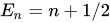

- If
for any nonzero constant
.
- The
-th excited state
.
- For even
is symmetric and nonzero at the origin.
- For odd
is antisymmetric and thus zero at the origin.
To find the 
- Guess some energy
- Integrate the Schrödinger equation. For example, use the central finite difference
- If
to some arbitrary number (say
, the wave function can be normalized after integration anyway) and use the symmetric property to find all remaining
.
- If
and
to some arbitrary number (say
, the wave function can be normalized after integration anyway) and find all remaining
- If
- Count the roots of
and refine the guess for the energy
- If there are
- If there are more than
- If there are

The energy-guessing can be done with the bisection method, and the process can be terminated when the energy difference is sufficiently small. Then one can take any energy in the interval to be the correct energy.
Sources and credits
This article is adapted from the Wikipedia article “Shooting method”, written by its contributors and licensed under CC BY-SA 4.0. Fathomly has changed the layout, removed citation markers, navigation and maintenance notices, and adjusted punctuation. This adapted version is shared under the same license. For references, see the original article.
Images, from Wikimedia Commons:
- Shooting method trajectories.svg by Nicoguaro, CC BY 4.0
- Shooting method error.svg by Nicoguaro, CC BY 4.0
- Shooting method.svg by Hersle, CC BY-SA 4.0
Fathomly is not affiliated with or endorsed by the Wikimedia Foundation. Spotted a problem? Tell us.