Segmentation-based object categorization
The image segmentation problem is concerned with partitioning an image into multiple regions according to some homogeneity criterion. This article is primarily concerned with graph theoretic approaches to image segmentation applying graph partitioning via minimum cut or maximum cut. Segmentation-based object categorization can be viewed as a specific case of spectral clustering applied to image segmentation.
01Applications of image segmentation
- Image compression
- Segment the image into homogeneous components, and use the most suitable compression algorithm for each component to improve compression.
- Medical diagnosis
- Automatic segmentation of MRI images for identification of cancerous regions.
- Mapping and measurement
- Automatic analysis of remote sensing data from satellites to identify and measure regions of interest.
- Transportation
- Partition a transportation network makes it possible to identify regions characterized by homogeneous traffic states.
02Segmentation using normalized cuts
Graph theoretic formulation
The set of points in an arbitrary feature space can be represented as a weighted undirected complete graph G = (V, E), where the nodes of the graph are the points in the feature space. The weight 


Normalized cuts
Let G = (V, E, w) be a weighted graph. Let 

Let:
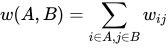


In the normalized cuts approach, for any cut 


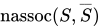
Since 

Computing a cut
The ncut algorithm
Let:
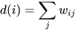
Also, let D be an 


After some algebraic manipulations, we get:

subject to the constraints:
, for some constant


Minimizing 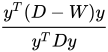


The partitioning algorithm:
- Given a set of features, set up a weighted graph
, compute the weight of each edge, and summarize the information in
and
- Solve
- Use the eigenvector with the second smallest eigenvalue to bipartition the graph (e.g. grouping according to sign).
- Decide if the current partition should be subdivided.
- Recursively partition the segmented parts, if necessary.
Computational Complexity
Solving a standard eigenvalue problem for all eigenvectors (using the QR algorithm, for instance) takes 

Since only one eigenvector, corresponding to the second smallest generalized eigenvalue, is used by the uncut algorithm, efficiency can be dramatically improved if the solve of the corresponding eigenvalue problem is performed in a matrix-free fashion, i.e., without explicitly manipulating with or even computing the matrix W, as, e.g., in the Lanczos algorithm. Matrix-free methods require only a function that performs a matrix-vector product for a given vector, on every iteration. For image segmentation, the matrix W is typically sparse, with a number of nonzero entries 
For high-resolution images, the second eigenvalue is often ill-conditioned, leading to slow convergence of iterative eigenvalue solvers, such as the Lanczos algorithm. Preconditioning is a key technology accelerating the convergence, e.g., in the matrix-free LOBPCG method. Computing the eigenvector using an optimally preconditioned matrix-free method takes
Software Implementations
scikit-learn uses LOBPCG from SciPy with algebraic multigrid preconditioning for solving the eigenvalue problem for the graph Laplacian to perform image segmentation via spectral graph partitioning as first proposed in and actually tested in and.
03OBJ CUT
OBJ CUT is an efficient method that automatically segments an object. The OBJ CUT method is a generic method, and therefore it is applicable to any object category model. Given an image D containing an instance of a known object category, e.g. cows, the OBJ CUT algorithm computes a segmentation of the object, that is, it infers a set of labels m.
Let m be a set of binary labels, and let 

(1)
The term 



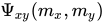
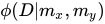
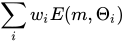
The best labeling 


(2)
Algorithm
- Given an image D, an object category is chosen, e.g. cows or horses.
- The corresponding LPS model is matched to D to obtain the samples
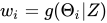
- The objective function given by equation (2) is determined by computing
and using
- The objective function is minimized using a single MINCUT operation to obtain the segmentation m.

04Other approaches
- Jigsaw approach
- Image parsing
- Interleaved segmentation
- LOCUS
- LayoutCRF
- Minimum spanning tree-based segmentation
Sources and credits
This article is adapted from the Wikipedia article “Segmentation-based object categorization”, written by its contributors and licensed under CC BY-SA 4.0. Fathomly has changed the layout, removed citation markers, navigation and maintenance notices, and adjusted punctuation. This adapted version is shared under the same license. For references, see the original article.
Fathomly is not affiliated with or endorsed by the Wikimedia Foundation. Spotted a problem? Tell us.