Encyclopedia

Second variation

Concept in differential calculus

Wikipedia contributorsAdapted for Fathomly · View authors

3 min read
Source updated September 17, 2025

In the calculus of variations, the second variation extends the idea of the second derivative test to functionals. Much like for functions, at a stationary point where the first derivative is zero, the second derivative determines the nature of the stationary point; it may be negative (if the point is a maximum point), positive (if a minimum) or zero (if a saddle point).

Via the second functional, it is possible to derive powerful necessary conditions for solving variational problems, such as the Legendre-Clebsch condition and the Jacobi necessary condition detailed below.

01Motivation

Much of the calculus of variations relies on the first variation, which is a generalization of the first derivative to a functional. An example of a class of variational problems is to find the function $y$ which minimizes the integral

$J[y]=\int _{a}^{b}f(x,y,y')dx$

on the interval $[a,b]$ ; $J$ here is a functional (a mapping which takes a function and returns a scalar). It is known that any smooth function $y$ which minimizes this functional satisfies the Euler-Lagrange equation

$f_{y}-{\frac {d}{dx}}f_{y'}=0.$

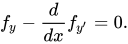
These solutions are stationary, but there is no guarantee that they are the type of extremum desired (completely analogously to the first derivative, they may be a minimum, maximum or saddle point). A test via the second variation would ensure that the solution is a minimum.

02Derivation

Take an extremum $y$ . The Taylor series of the integrand of our variational functional about a nearby point $y+\varepsilon h$ where $\varepsilon$ is small and $h$ is a smooth function which is zero at $a$ and $b$ is

$f(x,y,y')=f(x,y,y')+\varepsilon (hf_{y}+h'f_{y'})+{\frac {\varepsilon ^{2}}{2}}(h^{2}f_{yy}+2hh'f_{yy'}+h'^{2}f_{y'y'})+O(\varepsilon ^{3}).$

The first term of the series is the first variation, and the second is defined to be the second variation:

$\delta ^{2}J(h,y):=\int _{a}^{b}h^{2}f_{yy}+2hh'f_{yy'}+f_{y'y'}h'^{2}.$

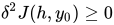
It can then be shown that $J$ has a local minimum at $y_{0}$ if it is stationary (i.e. the first variation is zero) and $\delta ^{2}J(h,y_{0})\geq 0$ for all $h$ .

03The Jacobi necessary condition

The accessory problem and Jacobi differential equation

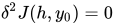
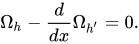
As discussed above, a minimum of the problem requires that $\delta ^{2}J(h,y_{0})\geq 0$ for all $h$ ; furthermore, the trivial solution $h=0$ gives $\delta ^{2}J(h,y_{0})=0$ . Thus consider $\delta ^{2}J(h,y_{0})$ can be considered as a variational problem in itself - this is called the accessory problem with integrand denoted $\Omega$ . The Jacobi differential equation is then the Euler-Lagrange equation for this accessory problem:

$\Omega _{h}-{\frac {d}{dx}}\Omega _{h'}=0.$

Conjugate points and the Jacobi necessary condition

As well as being easier to construct than the original Euler-Lagrange equation (due $h$ and $h'$ being at most quadratic) the Jacobi equation also expresses the conjugate points of the original variational problem in its solutions. A point $c$ is conjugate to the lower boundary $a$ if there is a nontrivial solution $h$ to the Jacobi differential equation with $h(a)=h(c)=0$ .

The Jacobi necessary condition then follows:

Let $y$ be an extremal for a variational integral on $[a,b]$ . Then a point $c\in (a,b)$ is a conjugate point of $a$ only if $f_{y'y'}(c,y,y')=0$ .

In particular, if $f$ satisfies the strengthened Legendre condition $f_{y'y'}>0$ , then $y$ is only an extremal if it has no conjugate points.

The Jacobi necessary condition is named after Carl Jacobi, who first utilized the solutions for the accessory problem in his article Zur Theorie der Variations-Rechnung und der Differential-Gleichungen, and the term 'accessory problem' was introduced by von Escherich.

04An example: shortest path on a sphere

As an example, the problem of finding a geodesic (shortest path) between two points on a sphere can be represented as the variational problem with functional

$J[y]=\int _{0}^{b}{\sqrt {\cos ^{2}y+y'^{2}}}dx.$

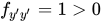
The equator of the sphere, $y=0$ minimizes this functional with $f_{y'y'}=1>0$ ; for this problem the Jacobi differential equation is

$h''+h=0$

which has solutions $h=A\sin(x)+B\cos(x)$ . If a solution satisfies $h(0)=0$ , then it must have the form $h=A\sin(x)$ . These functions have zeroes at $k\pi ,k\in \mathbb {Z}$ , and so the equator is only a solution if $b<\pi$ .

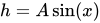
This makes intuitive sense; if one draws a great circle through two points on the sphere, there are two paths between them, one longer than the other. If $b>\pi$ , then we are going over halfway around the circle to get to the other point, and it would be quicker to get there in the other direction.

Watch videos about Second variationExplainers and documentaries on YouTube (opens in a new tab)

Sources and credits

This article is adapted from the Wikipedia article “Second variation”, written by its contributors and licensed under CC BY-SA 4.0. Fathomly has changed the layout, removed citation markers, navigation and maintenance notices, and adjusted punctuation. This adapted version is shared under the same license. For references, see the original article.

Fathomly is not affiliated with or endorsed by the Wikimedia Foundation. Spotted a problem? Tell us.