Encyclopedia

Quaternionic matrix

Concept in linear algebra

Wikipedia contributorsAdapted for Fathomly · View authors

2 min read
Source updated August 3, 2026

A quaternionic matrix is a matrix whose elements are quaternions.

01Matrix operations

The quaternions form a noncommutative ring, and therefore addition and multiplication can be defined for quaternionic matrices as for matrices over any ring.

Addition. The sum of two quaternionic matrices A and B is defined in the usual way by element-wise addition:

$(A+B)_{ij}=A_{ij}+B_{ij}.\,$

Multiplication. The product of two quaternionic matrices A and B also follows the usual definition for matrix multiplication. For it to be defined, the number of columns of A must equal the number of rows of B. Then the entry in the ith row and jth column of the product is the dot product of the ith row of the first matrix with the jth column of the second matrix. Specifically:

$(AB)_{ij}=\sum _{s}A_{is}B_{sj}.\,$

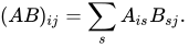
For example, for

$U={\begin{pmatrix}u_{11}&u_{12}\\u_{21}&u_{22}\\\end{pmatrix}},\quad V={\begin{pmatrix}v_{11}&v_{12}\\v_{21}&v_{22}\\\end{pmatrix}},$

the product is

$UV={\begin{pmatrix}u_{11}v_{11}+u_{12}v_{21}&u_{11}v_{12}+u_{12}v_{22}\\u_{21}v_{11}+u_{22}v_{21}&u_{21}v_{12}+u_{22}v_{22}\\\end{pmatrix}}.$

Since quaternionic multiplication is noncommutative, care must be taken to preserve the order of the factors when computing the product of matrices.

The identity for this multiplication is, as expected, the diagonal matrix I = diag(1, 1, ... , 1). Multiplication follows the usual laws of associativity and distributivity. The trace of a matrix is defined as the sum of the diagonal elements, but in general

$\operatorname {trace} (AB)\neq \operatorname {trace} (BA).$

Left scalar multiplication, and right scalar multiplication are defined by

$(cA)_{ij}=cA_{ij},\qquad (Ac)_{ij}=A_{ij}c.\,$

Again, since multiplication is not commutative some care must be taken in the order of the factors.

02Determinants

There is no natural way to define a determinant for (square) quaternionic matrices so that the values of the determinant are quaternions. Complex valued determinants can be defined however. The quaternion a + bi + cj + dk can be represented as the 2×2 complex matrix

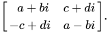
${\begin{bmatrix}~~a+bi&c+di\\-c+di&a-bi\end{bmatrix}}.$

This defines a map Ψ_mn from the m by n quaternionic matrices to the 2m by 2n complex matrices by replacing each entry in the quaternionic matrix by its 2 by 2 complex representation. The complex valued determinant of a square quaternionic matrix A is then defined as det(Ψ(A)). Many of the usual laws for determinants hold; in particular, an n by n matrix is invertible if and only if its determinant is nonzero.

03Hyperquaternionic representation

Due to the isomorphism $\mathbb {H} ^{\otimes 2}\simeq m(4,\mathbb {R} )$ where $m(4,\mathbb {R} )$ is a $4\times 4$ real matrix, a quaternion matrix can be represented as a hypercomplex number constituted by a tensor product of quaternion algebras called hyperquaternions

${\begin{aligned}\mathbb {H} ^{\otimes m}&=\mathbb {H} \otimes \mathbb {H} \otimes \cdots \otimes \mathbb {H} {\text{ }}(m{\text{ terms}})\\&=(i,j,k)\otimes (I,J,K)\otimes (l,m,n)\otimes \cdots \\\end{aligned}}$

where $(i,j,k),(I,J,K),(l,m,n)$ , etc. are commuting quaternionic systems. $i=i\otimes 1,J=1\otimes j,iJ=(i\otimes 1)(1\otimes j)$ , etc . Examples are: $M_{4\times 4}\mathbb {(H)} \simeq \mathbb {H} ^{\otimes 2}\otimes \mathbb {H} \simeq \mathbb {H} ^{\otimes 3}$ , $M_{16\times 16}\mathbb {(H)} \simeq \mathbb {H} ^{\otimes 4}\otimes \mathbb {H} \simeq \mathbb {H} ^{\otimes 5}$ .

A hyperconjugation is defined by $(\mathbb {H} ^{\otimes m})^{*}=(\mathbb {H} _{c}^{\otimes m})=\mathbb {H} _{c}\otimes \mathbb {H} _{c}\otimes \cdots \otimes \mathbb {H} _{c}$

where $\mathbb {H} _{c}$ is the quaternion conjugation hence, $(iJ)^{*}=(-i)(-J)=iJ$ . In particular, $(\mathbb {H} ^{\otimes 3})^{*}=[M_{4\times 4}\mathbb {(H)} ]_{c}^{T}$ where $[A\mathbb {(H)} ]_{c}^{T}$ is the transpose quaternion conjugate of the quaternionic matrix $A\mathbb {(H)}$ .

The unitary symplectic group $USp(n)$ is the group of quaternionic matrices $A\in M_{n\times n}\mathbb {(H)}$ such that $AA^{*}=A^{*}A=E_{n}$ .

Hyperquaternions are Clifford algebras $Cl_{p,q}\mathbb {(R)}$ having $n=p+q$ generators $e_{1},e_{2},...,e_{n}$ multipying according to $e_{i}e_{j}+e_{j}e_{i}=0$ $(i\neq j)$ with $e_{i}^{2}=+1$ ( $p$ generators) and $e_{i}^{2}=-1$ ( $q$ generators) . One has $\mathbb {H} \simeq Cl_{0,2}\mathbb {(R)} ,\mathbb {H} ^{\otimes 3}\simeq Cl_{2,4}\mathbb {(R)} ,\mathbb {H} ^{\otimes 5}\simeq Cl_{4,6}\mathbb {(R)}$ . A basis of $\mathbb {H} ^{\otimes 2}\simeq M_{4\times 4}\mathbb {(R)}$ is given by

${\begin{aligned}e_{0}&=j\otimes 1=j={\begin{bmatrix}0&0&-1&0\\0&0&0&-1\\1&0&0&0\\0&1&0&0\\\end{bmatrix}},e_{1}=k\otimes i=kI={\begin{bmatrix}0&0&1&0\\0&0&0&-1\\1&0&0&0\\0&-1&0&0\\\end{bmatrix}},\\e_{2}&=k\otimes j=kJ={\begin{bmatrix}-1&0&0&0\\0&-1&0&0\\0&0&1&0\\0&0&0&1\\\end{bmatrix}},e_{3}=k\otimes k=kK={\begin{bmatrix}0&0&0&-1\\0&0&-1&0\\0&-1&0&0\\-1&0&0&0\\\end{bmatrix}}.\\\end{aligned}}$

04Applications

Quaternionic matrices are used in quantum mechanics and in the treatment of multibody problems.

Watch videos about Quaternionic matrixExplainers and documentaries on YouTube (opens in a new tab)

Sources and credits

This article is adapted from the Wikipedia article “Quaternionic matrix”, written by its contributors and licensed under CC BY-SA 4.0. Fathomly has changed the layout, removed citation markers, navigation and maintenance notices, and adjusted punctuation. This adapted version is shared under the same license. For references, see the original article.

Fathomly is not affiliated with or endorsed by the Wikimedia Foundation. Spotted a problem? Tell us.