Encyclopedia

Q-function

Statistics function

Wikipedia contributorsAdapted for Fathomly · View authors

5 min read
Source updated July 11, 2026

Image credit is listed at the end of this article.

In statistics, the Q-function is the tail distribution function of the standard normal distribution. In other words, $Q(x)$ is the probability that a normal (Gaussian) random variable will obtain a value larger than $x$ standard deviations. Equivalently, $Q(x)$ is the probability that a standard normal random variable takes a value larger than $x$ .

If $Y$ is a Gaussian random variable with mean $\mu$ and variance $\sigma ^{2}$ , then $X={\frac {Y-\mu }{\sigma }}$ is standard normal and

$P(Y>y)=P(X>x)=Q(x)$

where $x={\frac {y-\mu }{\sigma }}$ .

Other definitions of the Q-function, all of which are simple transformations of the normal cumulative distribution function, are also used occasionally.

Because of its relation to the cumulative distribution function of the normal distribution, the Q-function can also be expressed in terms of the error function, which is an important function in applied mathematics and physics.

01Definition and basic properties

Formally, the Q-function is defined as

$Q(x)={\frac {1}{\sqrt {2\pi }}}\int _{x}^{\infty }\exp \left(-{\frac {u^{2}}{2}}\right)\,du.$

Thus,

$Q(x)=1-Q(-x)=1-\Phi (x)\,\!,$

where $\Phi (x)$ is the cumulative distribution function of the standard normal Gaussian distribution.

The Q-function can be expressed in terms of the error function, or the complementary error function, as

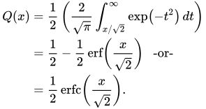
${\begin{aligned}Q(x)&={\frac {1}{2}}\left({\frac {2}{\sqrt {\pi }}}\int _{x/{\sqrt {2}}}^{\infty }\exp \left(-t^{2}\right)\,dt\right)\\&={\frac {1}{2}}-{\frac {1}{2}}\operatorname {erf} \left({\frac {x}{\sqrt {2}}}\right)~~{\text{ -or-}}\\&={\frac {1}{2}}\operatorname {erfc} \left({\frac {x}{\sqrt {2}}}\right).\end{aligned}}$

An alternative form of the Q-function known as Craig's formula, after its discoverer, is expressed as:

$Q(x)={\frac {1}{\pi }}\int _{0}^{\frac {\pi }{2}}\exp \left(-{\frac {x^{2}}{2\sin ^{2}\theta }}\right)d\theta .$

The above proper integral form of Q-function, has been incorrectly credited to Craig. This form of Q-function was implied in earlier works by Wiesten , and explicitly stated by Pawula, Rice and Roberts.

This expression is valid only for positive values of x, but it can be used in conjunction with Q(x) = 1 − Q(−x) to obtain Q(x) for negative values. This form is advantageous in that the range of integration is fixed and finite.

Craig's formula was later extended by Behnad (2020) for the Q-function of the sum of two non-negative variables, as follows:

$Q(x+y)={\frac {1}{\pi }}\int _{0}^{\frac {\pi }{2}}\exp \left(-{\frac {x^{2}}{2\sin ^{2}\theta }}-{\frac {y^{2}}{2\cos ^{2}\theta }}\right)d\theta ,\quad x,y\geqslant 0.$

02Bounds and approximations

The Q-function is not an elementary function. However, it can be upper and lower bounded as,

$\left({\frac {x}{1+x^{2}}}\right)\phi (x)<Q(x)<{\frac {\phi (x)}{x}},\qquad x>0,$

where $\phi (x)$ is the density function of the standard normal distribution, and the bounds become increasingly tight for large x.

Using the substitution v =u²/2, the upper bound is derived as follows:

$Q(x)=\int _{x}^{\infty }\phi (u)\,du<\int _{x}^{\infty }{\frac {u}{x}}\phi (u)\,du=\int _{\frac {x^{2}}{2}}^{\infty }{\frac {e^{-v}}{x{\sqrt {2\pi }}}}\,dv=-{\biggl .}{\frac {e^{-v}}{x{\sqrt {2\pi }}}}{\biggr |}_{\frac {x^{2}}{2}}^{\infty }={\frac {\phi (x)}{x}}.$

Similarly, using $\phi '(u)=-u\phi (u)$ and the quotient rule,

$\left(1+{\frac {1}{x^{2}}}\right)Q(x)=\int _{x}^{\infty }\left(1+{\frac {1}{x^{2}}}\right)\phi (u)\,du>\int _{x}^{\infty }\left(1+{\frac {1}{u^{2}}}\right)\phi (u)\,du=-{\biggl .}{\frac {\phi (u)}{u}}{\biggr |}_{x}^{\infty }={\frac {\phi (x)}{x}}.$

Solving for Q(x) provides the lower bound.

The geometric mean of the upper and lower bound gives a suitable approximation for $Q(x)$ :

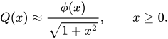
$Q(x)\approx {\frac {\phi (x)}{\sqrt {1+x^{2}}}},\qquad x\geq 0.$

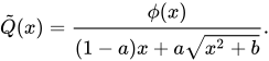
Tighter bounds and approximations of $Q(x)$ can also be obtained by optimizing the following expression

${\tilde {Q}}(x)={\frac {\phi (x)}{(1-a)x+a{\sqrt {x^{2}+b}}}}.$

For $x\geq 0$ , the best upper bound is given by $a=0.344$ and $b=5.334$ with maximum absolute relative error of 0.44%. Likewise, the best approximation is given by $a=0.339$ and $b=5.510$ with maximum absolute relative error of 0.27%. Finally, the best lower bound is given by $a=1/\pi$ and $b=2\pi$ with maximum absolute relative error of 1.17%.

The Chernoff bound of the Q-function is

$Q(x)\leq e^{-{\frac {x^{2}}{2}}},\qquad x>0$

Improved exponential bounds and a pure exponential approximation are

$Q(x)\leq {\tfrac {1}{4}}e^{-x^{2}}+{\tfrac {1}{4}}e^{-{\frac {x^{2}}{2}}}\leq {\tfrac {1}{2}}e^{-{\frac {x^{2}}{2}}},\qquad x>0$

$Q(x)\approx {\frac {1}{12}}e^{-{\frac {x^{2}}{2}}}+{\frac {1}{4}}e^{-{\frac {2}{3}}x^{2}},\qquad x>0$

The above were generalized by Tanash & Riihonen (2020), who showed that $Q(x)$ can be accurately approximated or bounded by

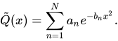
${\tilde {Q}}(x)=\sum _{n=1}^{N}a_{n}e^{-b_{n}x^{2}}.$

In particular, they presented a systematic methodology to solve the numerical coefficients $\{(a_{n},b_{n})\}_{n=1}^{N}$ that yield a minimax approximation or bound: $Q(x)\approx {\tilde {Q}}(x)$ , $Q(x)\leq {\tilde {Q}}(x)$ , or $Q(x)\geq {\tilde {Q}}(x)$ for $x\geq 0$ . With the example coefficients tabulated in the paper for $N=20$ , the relative and absolute approximation errors are less than $2.831\cdot 10^{-6}$ and $1.416\cdot 10^{-6}$ , respectively. The coefficients $\{(a_{n},b_{n})\}_{n=1}^{N}$ for many variations of the exponential approximations and bounds up to $N=25$ have been released to open access as a comprehensive dataset.

Another approximation of $Q(x)$ for $x\in [0,\infty )$ is given by Karagiannidis & Lioumpas (2007) who showed for the appropriate choice of parameters $\{A,B\}$ that

$f(x;A,B)={\frac {\left(1-e^{-Ax}\right)e^{-x^{2}}}{B{\sqrt {\pi }}x}}\approx \operatorname {erfc} \left(x\right).$

The absolute error between $f(x;A,B)$ and $\operatorname {erfc} (x)$ over the range $[0,R]$ is minimized by evaluating

$\{A,B\}={\underset {\{A,B\}}{\arg \min }}{\frac {1}{R}}\int _{0}^{R}|f(x;A,B)-\operatorname {erfc} (x)|dx.$

Using $R=20$ and numerically integrating, they found the minimum error occurred when $\{A,B\}=\{1.98,1.135\},$ which gave a good approximation for $\forall x\geq 0.$

Substituting these values and using the relationship between $Q(x)$ and $\operatorname {erfc} (x)$ from above gives

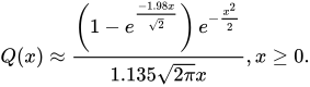
$Q(x)\approx {\frac {\left(1-e^{\frac {-1.98x}{\sqrt {2}}}\right)e^{-{\frac {x^{2}}{2}}}}{1.135{\sqrt {2\pi }}x}},x\geq 0.$

Alternative coefficients are also available for the above 'Karagiannidis-Lioumpas approximation' for tailoring accuracy for a specific application or transforming it into a tight bound.

A tighter and more tractable approximation of $Q(x)$ for positive arguments $x\in [0,\infty )$ is given by López-Benítez & Casadevall (2011) based on a second-order exponential function:

$Q(x)\approx e^{-ax^{2}-bx-c},\qquad x\geq 0.$

The fitting coefficients $(a,b,c)$ can be optimized over any desired range of arguments in order to minimize the sum of square errors ( $a=0.3842$ , $b=0.7640$ , $c=0.6964$ for $x\in [0,20]$ ) or minimize the maximum absolute error ( $a=0.4920$ , $b=0.2887$ , $c=1.1893$ for $x\in [0,20]$ ). This approximation offers some benefits such as a good trade-off between accuracy and analytical tractability (for example, the extension to any arbitrary power of $Q(x)$ is trivial and does not alter the algebraic form of the approximation).

A pair of tight lower and upper bounds on the Gaussian Q-function for positive arguments $x\in [0,\infty )$ was introduced by Abreu (2012) based on a simple algebraic expression with only two exponential terms:

$Q(x)\geq {\frac {1}{12}}e^{-x^{2}}+{\frac {1}{{\sqrt {2\pi }}(x+1)}}e^{-x^{2}/2},\qquad x\geq 0,$

$Q(x)\leq {\frac {1}{50}}e^{-x^{2}}+{\frac {1}{2(x+1)}}e^{-x^{2}/2},\qquad x\geq 0.$

These bounds are derived from a unified form $Q_{\mathrm {B} }(x;a,b)={\frac {\exp(-x^{2})}{a}}+{\frac {\exp(-x^{2}/2)}{b(x+1)}}$ , where the parameters $a$ and $b$ are chosen to satisfy specific conditions ensuring the lower ( $a_{\mathrm {L} }=12$ , $b_{\mathrm {L} }={\sqrt {2\pi }}$ ) and upper ( $a_{\mathrm {U} }=50$ , $b_{\mathrm {U} }=2$ ) bounding properties. The resulting expressions are notable for their simplicity and tightness, offering a favorable trade-off between accuracy and mathematical tractability. These bounds are particularly useful in theoretical analysis, such as in communication theory over fading channels. Additionally, they can be extended to bound $Q^{n}(x)$ for positive integers $n$ using the binomial theorem, maintaining their simplicity and effectiveness.

03Inverse Q

The inverse Q-function can be related to the inverse error functions:

$Q^{-1}(y)={\sqrt {2}}\ \mathrm {erf} ^{-1}(1-2y)={\sqrt {2}}\ \mathrm {erfc} ^{-1}(2y)$

The function $Q^{-1}(y)$ finds application in digital communications. It is usually expressed in dB and generally called Q-factor:

$\mathrm {Q{\text{-}}factor} =20\log _{10}\!\left(Q^{-1}(y)\right)\!~\mathrm {dB}$

where y is the bit-error rate (BER) of the digitally modulated signal under analysis. For instance, for quadrature phase-shift keying (QPSK) in additive white Gaussian noise, the Q-factor defined above coincides with the value in dB of the signal to noise ratio that yields a bit error rate equal to y.

04Values

The Q-function is well tabulated and can be computed directly in most of the mathematical software packages such as R and those available in Python, MATLAB and Mathematica. Some values of the Q-function are given below for reference.

Q(0.0)	0.500000000	1/2.0000
Q(0.1)	0.460172163	1/2.1731
Q(0.2)	0.420740291	1/2.3768
Q(0.3)	0.382088578	1/2.6172
Q(0.4)	0.344578258	1/2.9021
Q(0.5)	0.308537539	1/3.2411
Q(0.6)	0.274253118	1/3.6463
Q(0.7)	0.241963652	1/4.1329
Q(0.8)	0.211855399	1/4.7202
Q(0.9)	0.184060125	1/5.4330

Q(1.0)	0.158655254	1/6.3030
Q(1.1)	0.135666061	1/7.3710
Q(1.2)	0.115069670	1/8.6904
Q(1.3)	0.096800485	1/10.3305
Q(1.4)	0.080756659	1/12.3829
Q(1.5)	0.066807201	1/14.9684
Q(1.6)	0.054799292	1/18.2484
Q(1.7)	0.044565463	1/22.4389
Q(1.8)	0.035930319	1/27.8316
Q(1.9)	0.028716560	1/34.8231

Q(2.0)	0.022750132	1/43.9558
Q(2.1)	0.017864421	1/55.9772
Q(2.2)	0.013903448	1/71.9246
Q(2.3)	0.010724110	1/93.2478
Q(2.4)	0.008197536	1/121.9879
Q(2.5)	0.006209665	1/161.0393
Q(2.6)	0.004661188	1/214.5376
Q(2.7)	0.003466974	1/288.4360
Q(2.8)	0.002555130	1/391.3695
Q(2.9)	0.001865813	1/535.9593

Q(3.0)	0.001349898	1/740.7967
Q(3.1)	0.000967603	1/1033.4815
Q(3.2)	0.000687138	1/1455.3119
Q(3.3)	0.000483424	1/2068.5769
Q(3.4)	0.000336929	1/2967.9820
Q(3.5)	0.000232629	1/4298.6887
Q(3.6)	0.000159109	1/6285.0158
Q(3.7)	0.000107800	1/9276.4608
Q(3.8)	0.000072348	1/13822.0738
Q(3.9)	0.000048096	1/20791.6011
Q(4.0)	0.000031671	1/31574.3855

05Generalization to high dimensions

The Q-function can be generalized to higher dimensions:

$Q(\mathbf {x} )=\mathbb {P} (\mathbf {X} \geq \mathbf {x} ),$

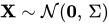
where $\mathbf {X} \sim {\mathcal {N}}(\mathbf {0} ,\,\Sigma )$ follows the multivariate normal distribution with covariance $\Sigma$ and the threshold is of the form $\mathbf {x} =\gamma \Sigma \mathbf {l} ^{*}$ for some positive vector $\mathbf {l} ^{*}>\mathbf {0}$ and positive constant $\gamma >0$ . As in the one dimensional case, there is no simple analytical formula for the Q-function. Nevertheless, the Q-function can be approximated arbitrarily well as $\gamma$ becomes larger and larger.

Watch videos about Q-functionExplainers and documentaries on YouTube (opens in a new tab)

Sources and credits

This article is adapted from the Wikipedia article “Q-function”, written by its contributors and licensed under CC BY-SA 4.0. Fathomly has changed the layout, removed citation markers, navigation and maintenance notices, and adjusted punctuation. This adapted version is shared under the same license. For references, see the original article.

Images, from Wikimedia Commons:

Q-function.png by Zvika, Public domain
Q function complex plot plotted with Mathematica 13.1 ComplexPlot3D.svg by WalkingRadiance, CC BY-SA 4.0
Q-factor vs BER.png by Paolostar, CC BY-SA 4.0

Fathomly is not affiliated with or endorsed by the Wikimedia Foundation. Spotted a problem? Tell us.