Encyclopedia

Pulsatile flow

Flow with periodic variations

Wikipedia contributorsAdapted for Fathomly · View authors

4 min read
Source updated May 13, 2026

In fluid dynamics, a flow with periodic variations is known as pulsatile flow, or as Womersley flow. The flow profiles was first derived by John R. Womersley (1907-1958) in his work with blood flow in arteries. The cardiovascular system of chordate animals is a very good example where pulsatile flow is found, but pulsatile flow is also observed in engines and hydraulic systems, as a result of rotating mechanisms pumping the fluid.

01Equation

The pulsatile flow profile is given in a straight pipe by

$u(r,t)=\mathrm {Re} \left\{\sum _{n=0}^{N}{\frac {i\,P'_{n}}{\rho \,n\,\omega }}\left[1-{\frac {J_{0}(\alpha \,n^{1/2}\,i^{3/2}\,{\frac {r}{R}})}{J_{0}(\alpha \,n^{1/2}\,i^{3/2})}}\right]e^{in\omega t}\right\}\,,$

where:

u	is the longitudinal flow velocity,
r	is the radial coordinate,
t	is time,
α	is the dimensionless Womersley number,
ω	is the angular frequency of the first harmonic of a Fourier series of an oscillatory pressure gradient,
n	are the natural numbers,
P'_n	is the pressure gradient magnitude for the frequency nω,
ρ	is the fluid density,
μ	is the dynamic viscosity,
R	is the pipe radius,
J₀(·)	is the Bessel function of first kind and order zero,
i	is the imaginary number, and
Re{·}	is the real part of a complex number.

02Properties

Womersley number

The pulsatile flow profile changes its shape depending on the Womersley number

$\alpha =R\left({\frac {\omega \rho }{\mu }}\right)^{1/2}.$

For $\alpha \lesssim 2$ , viscous forces dominate the flow, and the pulse is considered quasi-static with a parabolic profile. For $\alpha \gtrsim 2$ , the inertial forces are dominant in the central core, whereas viscous forces dominate near the boundary layer. Thus, the velocity profile gets flattened, and phase between the pressure and velocity waves gets shifted towards the core.

Function limits

Lower limit

The Bessel function at its lower limit becomes

$\lim _{z\to \infty }J_{0}(z)=1-{\frac {z^{2}}{4}}\,,$

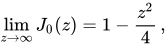
which converges to the Hagen-Poiseuille flow profile for steady flow for

$\lim _{n\to 0}u(r,t)=-{\frac {P'_{0}}{4\mu }}\left(R^{2}-r^{2}\right),$

or to a quasi-static pulse with parabolic profile when

$\lim _{\alpha \to 0}u(r,t)=\mathrm {Re} \left\{-\sum _{n=0}^{N}{\frac {P'_{n}}{4\mu }}(R^{2}-r^{2})\,e^{in\omega t}\right\}=-\sum _{n=0}^{N}{\frac {P'_{n}}{4\mu }}(R^{2}-r^{2})\,\cos(n\omega t)\,.$

In this case, the function is real, because the pressure and velocity waves are in phase.

Upper limit

The Bessel function at its upper limit becomes

$\lim _{z\to \infty }J_{0}(z\,i)={\frac {e^{z}}{\sqrt {2\pi \,z}}}\,,$

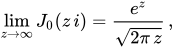
which converges to

$\lim _{z\to \infty }u(r,t)=\mathrm {Re} \left\{\sum _{n=0}^{N}{\frac {i\,P'_{n}}{\rho \,n\,\omega }}\left[1-e^{\alpha \,n^{1/2}\,i^{1/2}\left({\frac {r}{R}}-1\right)}\right]e^{in\omega t}\right\}=-\sum _{n=0}^{N}{\frac {\,P'_{n}}{\rho \,n\,\omega }}\left[1-e^{\alpha \,n^{1/2}\left({\frac {r}{R}}-1\right)}\right]\sin(n\,\omega \,t)\,.$

This is highly reminiscent of the Stokes layer on an oscillating flat plate, or the skin-depth penetration of an alternating magnetic field into an electrical conductor. On the surface, $u(r=R,t)=0$ , but the exponential term becomes negligible once $\alpha (1-r/R)$ becomes large, and the velocity profile becomes almost constant and independent of the viscosity. Thus, the flow simply oscillates as a plug profile in time according to the pressure gradient

$\rho {\frac {\partial u}{\partial t}}=-\sum _{n=0}^{N}P'_{n}\,.$

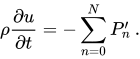
However, close to the walls, in a layer of thickness ${\mathcal {O}}(\alpha ^{-1})$ , the velocity adjusts rapidly to zero. Furthermore, the phase of the time oscillation varies quickly with position across the layer. The exponential decay of the higher frequencies is faster.

03Derivation

For deriving the analytical solution of this non-stationary flow-velocity profile, the following assumptions are taken:

The fluid is homogeneous, incompressible and Newtonian;
The tube wall is rigid and circular;
Motion is laminar, axisymmetric, and parallel to the tube's axis;
The boundary conditions are axisymmetry at the centre, and no-slip on the wall;
The pressure gradient is a periodic function that drives the fluid; and
Gravitation has no effect on the fluid.

Thus, the Navier-Stokes equation and the continuity equation are simplified as

$\rho {\frac {\partial u}{\partial t}}=-{\frac {\partial p}{\partial x}}+\mu \left({\frac {\partial ^{2}u}{\partial r^{2}}}+{\frac {1}{r}}{\frac {\partial u}{\partial r}}\right)\,$

and

${\frac {\partial u}{\partial x}}=0,$

respectively. The pressure gradient driving the pulsatile flow is decomposed in Fourier series,

${\frac {\partial p}{\partial x}}(t)=\sum _{n=0}^{N}P'_{n}e^{in\omega t},$

where $i$ is the imaginary number, $\omega$ is the angular frequency of the first harmonic (i.e., $n=1$ ), and $P'_{n}$ are the amplitudes of each harmonic $n$ . $P'_{0}$ (standing for $n=0$ ) is the steady-state pressure gradient, whose sign is opposed to the steady-state velocity (i.e., a negative pressure gradient yields positive flow). Similarly, the velocity profile is also decomposed in Fourier series in phase with the pressure gradient, because the fluid is incompressible,

$u(r,t)=\sum _{n=0}^{N}U_{n}e^{in\omega t},$

where $U_{n}$ are the amplitudes of each harmonic of the periodic function, and the steady component ( $n=0$ ) is simply Poiseuille flow

$U_{0}=-{\frac {P'_{0}}{4\mu }}\left(R^{2}-r^{2}\right).$

Thus, the Navier-Stokes equation for each harmonic reads as

$i\rho n\omega U_{n}=-P'_{n}+\mu \left({\frac {\partial ^{2}U_{n}}{\partial r^{2}}}+{\frac {1}{r}}{\frac {\partial U_{n}}{\partial r}}\right).$

With the boundary conditions satisfied, the general solution of this ordinary differential equation for the oscillatory part ( $n\geq 1$ ) is

$U_{n}(r)=A_{n}\,J_{0}\left(\alpha \,{\frac {r}{R}}n^{1/2}\,i^{3/2}\right)+B_{n}\,Y_{0}\left(\alpha \,{\frac {r}{R}}n^{1/2}\,i^{3/2}\right)+{\frac {i\,P'_{n}}{\rho \,n\,\omega }}\,,$

where $J_{0}(\cdot )$ is the Bessel function of first kind and order zero, $Y_{0}(\cdot )$ is the Bessel function of second kind and order zero, $A_{n}$ and $B_{n}$ are arbitrary constants, and $\alpha =R\surd (\omega \rho /\mu )$ is the dimensionless Womersley number. The axisymmetric boundary condition ( $\partial U_{n}/\partial r|_{r=0}=0$ ) is applied to show that $B_{n}=0$ for the derivative of above equation to be valid, as the derivatives $J_{0}'$ and $Y_{0}'$ approach infinity. Next, the wall non-slip boundary condition ( $U_{n}(R)=0$ ) yields

$A_{n}=-{\frac {i\,P'_{n}}{\rho \,n\,\omega }}{\frac {1}{J_{0}\left(\alpha \,n^{1/2}\,i^{3/2}\right)}}.$

Hence, the amplitudes of the velocity profile of the harmonic $n$ become

$U_{n}(r)={\frac {i\,P'_{n}}{\rho \,n\,\omega }}\left[1-{\frac {J_{0}(\alpha \,n^{1/2}\,i^{3/2}\,{\frac {r}{R}})}{J_{0}(\alpha \,n^{1/2}\,i^{3/2})}}\right]={\frac {i\,P'_{n}}{\rho \,n\,\omega }}\left[1-{\frac {J_{0}(\Lambda _{n}\,{\frac {r}{R}})}{J_{0}(\Lambda _{n})}}\right],$

where $\Lambda _{n}=\alpha \,n^{1/2}\,i^{3/2}$ is used for simplification. The velocity profile itself is obtained by taking the real part of the complex function resulted from the summation of all harmonics of the pulse,

$u(r,t)={\frac {P'_{0}}{4\mu }}\left(R^{2}-r^{2}\right)+\mathrm {Re} \left\{\sum _{n=1}^{N}{\frac {i\,P'_{n}}{\rho \,n\,\omega }}\left[1-{\frac {J_{0}(\Lambda _{n}\,{\frac {r}{R}})}{J_{0}(\Lambda _{n})}}\right]e^{in\omega t}\right\}.$

Flow rate

Flow rate is obtained by integrating the velocity field on the cross-section. Since,

${\frac {d}{dx}}\left[x^{p}J_{p}(a\,x)\right]=a\,x^{p}J_{p-1}(a\,x)\quad \Rightarrow \quad {\frac {d}{dx}}\left[x\,J_{1}(a\,x)\right]=a\,xJ_{0}(a\,x)\,,$

then

$Q(t)=\iint u(r,t)\,dA=\mathrm {Re} \left\{\pi \,R^{2}\,\sum _{n=1}^{N}{\frac {i\,P'_{n}}{\rho \,n\,\omega }}\left[1-{\frac {2}{\Lambda _{n}}}{\frac {J_{1}(\Lambda _{n})}{J_{0}(\Lambda _{n})}}\right]e^{in\omega t}\right\}.$

Velocity profile

To compare the shape of the velocity profile, it can be assumed that

$u(r,t)=f(r)\,{\frac {Q(t)}{A}}\,,$

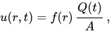
where

$f(r)={\frac {u(r,t)}{\frac {Q(t)}{A}}}=\mathrm {Re} \left\{\sum _{n=1}^{N}\left[{\frac {\Lambda _{n}\,J_{0}(\Lambda _{n})-\Lambda _{n}\,J_{0}(\Lambda _{n}\,{\frac {r}{R}})}{\Lambda _{n}\,J_{0}(\Lambda _{n})-2\,J_{1}(\Lambda _{n})}}\right]\right\}$

is the shape function. It is important to notice that this formulation ignores the inertial effects. The velocity profile approximates a parabolic or plug profile, for low or high Womersley numbers, respectively.

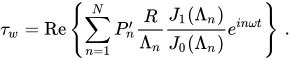
Wall shear stress

For straight pipes, wall shear stress is

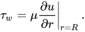
$\tau _{w}=\mu \left.{\frac {\partial u}{\partial r}}\right|_{r=R}\,.$

The derivative of a Bessel function is

${\frac {\partial }{\partial x}}\left[x^{-p}J_{-p}(a\,x)\right]=a\,x^{-p}J_{p+1}(a\,x)\quad \Rightarrow \quad {\frac {\partial }{\partial x}}\left[J_{0}(a\,x)\right]=-a\,J_{1}(a\,x)\,.$

Hence,

$\tau _{w}=\mathrm {Re} \left\{\sum _{n=1}^{N}P'_{n}{\frac {R}{\Lambda _{n}}}{\frac {J_{1}(\Lambda _{n})}{J_{0}(\Lambda _{n})}}e^{in\omega t}\right\}\,.$

Centre-line velocity

If the pressure gradient $P'_{n}$ is not measured, it can still be obtained by measuring the velocity at the centre line. The measured velocity has only the real part of the full expression in the form of

${\tilde {u}}(t)=\mathrm {Re} (u(0,t))\equiv \sum _{n=1}^{N}{\tilde {U}}_{n}\,\cos(n\,\omega \,t)\,.$

Noting that $J_{0}(0)=1$ , the full physical expression becomes

$u(0,t)=\mathrm {Re} \left\{\sum _{n=1}^{N}{\frac {i\,P'_{n}}{\rho \,n\,\omega }}\left[{\frac {J_{0}(\Lambda _{n})-1}{J_{0}(\Lambda _{n})}}\right]e^{in\omega t}\right\}$

at the centre line. The measured velocity is compared with the full expression by applying some properties of complex numbers. For any product of complex numbers $C=AB$ , the amplitude and phase have the relations $|C|=|A||B|$ and $\phi _{C}=\phi _{A}+\phi _{B}$ , respectively. Hence,

${\tilde {U}}_{n}=\left|{\frac {i\,P'_{n}}{\rho \,n\,\omega }}\left[{\frac {J_{0}(\Lambda _{n})-1}{J_{0}(\Lambda _{n})}}\right]\right|\quad \Rightarrow \quad P'_{n}={\tilde {U}}_{n}\left|i\,\rho \,n\,\omega \left[{\frac {J_{0}(\Lambda _{n})}{1-J_{0}(\Lambda _{n})}}\right]\right|$

and

${\tilde {\phi }}=0=\phi _{P'_{n}}+\phi _{U_{n}}\quad \Rightarrow \quad \phi _{P'_{n}}=\operatorname {phase} \left({\frac {i}{\rho \,n\,\omega }}\left[{\frac {1-J_{0}(\Lambda _{n})}{J_{0}(\Lambda _{n})}}\right]\right)\,,$

which finally yield

${\frac {1}{\rho }}{\frac {\partial p}{\partial x}}=\sum _{n=1}^{N}{\tilde {U}}_{n}\left|i\,\rho \,n\,\omega \left[{\frac {J_{0}(\Lambda _{n})}{1-J_{0}(\Lambda _{n})}}\right]\right|\,\cos \left\{n\,\omega \,t+\operatorname {phase} \left({\frac {i}{\rho \,n\,\omega }}\left[{\frac {1-J_{0}(\Lambda _{n})}{J_{0}(\Lambda _{n})}}\right]\right)\right\}\,.$

Watch videos about Pulsatile flowExplainers and documentaries on YouTube (opens in a new tab)

Sources and credits

This article is adapted from the Wikipedia article “Pulsatile flow”, written by its contributors and licensed under CC BY-SA 4.0. Fathomly has changed the layout, removed citation markers, navigation and maintenance notices, and adjusted punctuation. This adapted version is shared under the same license. For references, see the original article.

Images, from Wikimedia Commons:

Womersley Flow Profile.svg by Rudolf Hellmuth, CC BY-SA 4.0
Comparison of velocity profile of Womersley flow.svg by Rudolf Hellmuth, CC BY-SA 4.0

Fathomly is not affiliated with or endorsed by the Wikimedia Foundation. Spotted a problem? Tell us.

Pulsatile flow

01Equation

02Properties

Womersley number

Function limits

Lower limit

Upper limit

03Derivation

Flow rate

Velocity profile

Wall shear stress

Centre-line velocity

Sources and credits

Related topics

Circulatory system

Hemodynamics

Womersley number