Encyclopedia

Power iteration

Eigenvalue algorithm

Wikipedia contributorsAdapted for Fathomly · View authors

4 min read
Source updated July 14, 2026

In mathematics, power iteration (also known as the power method) is an eigenvalue algorithm: given a diagonalizable matrix $A$ , the algorithm will produce a number $\lambda$ , which is the greatest (in absolute value) eigenvalue of $A$ , and a nonzero vector $v$ , which is a corresponding eigenvector of $\lambda$ , that is, $Av=\lambda v$ . The algorithm is also known as the Von Mises iteration.

Power iteration is a very simple algorithm, but it may converge slowly. The most time-consuming operation of the algorithm is the multiplication of matrix $A$ by a vector, so it is effective for a very large sparse matrix with appropriate implementation. The speed of convergence is like $(\lambda _{2}/\lambda _{1})^{k}$ where $k$ is the number of iterations, and $\lambda _{1}$ and $\lambda _{2}$ are, respectively, the eigenvalue of largest absolute value and an eigenvalue of second-largest absolute value (see a later section). In other words, convergence is exponential with base being the spectral gap.

01The method

The power iteration algorithm starts with a vector $b_{0}$ , which may be an approximation to the dominant eigenvector or a random vector. The method is described by the recurrence relation

$b_{k+1}={\frac {Ab_{k}}{\lVert Ab_{k}\rVert }}$

So, at every iteration, the vector $b_{k}$ is multiplied by the matrix $A$ and normalized.

If we assume $A$ has an eigenvalue that is strictly greater in magnitude than its other eigenvalues, i.e.,

$\left\vert \lambda _{1}\right\vert >\left\vert \lambda _{2}\right\vert \geq \ldots \geq \left\vert \lambda _{n}\right\vert \geq 0$

and the starting vector $b_{0}$ has a nonzero component in the direction of an eigenvector associated with the dominant eigenvalue, then a subsequence $\left(b_{k}\right)$ converges to an eigenvector associated with the dominant eigenvalue.

Without the two assumptions above, the sequence $\left(b_{k}\right)$ does not necessarily converge. In this sequence,

$b_{k}=e^{i\phi _{k}}v_{1}+r_{k}$ ,

where $v_{1}$ is an eigenvector associated with the dominant eigenvalue, and $\|r_{k}\|\rightarrow 0$ . The presence of the term $e^{i\phi _{k}}$ implies that $\left(b_{k}\right)$ does not converge unless $e^{i\phi _{k}}=1$ . Under the two assumptions listed above, the sequence $\left(\mu _{k}\right)$ defined by

$\mu _{k}={\frac {b_{k}^{*}Ab_{k}}{b_{k}^{*}b_{k}}}$

converges to the dominant eigenvalue (with Rayleigh quotient).

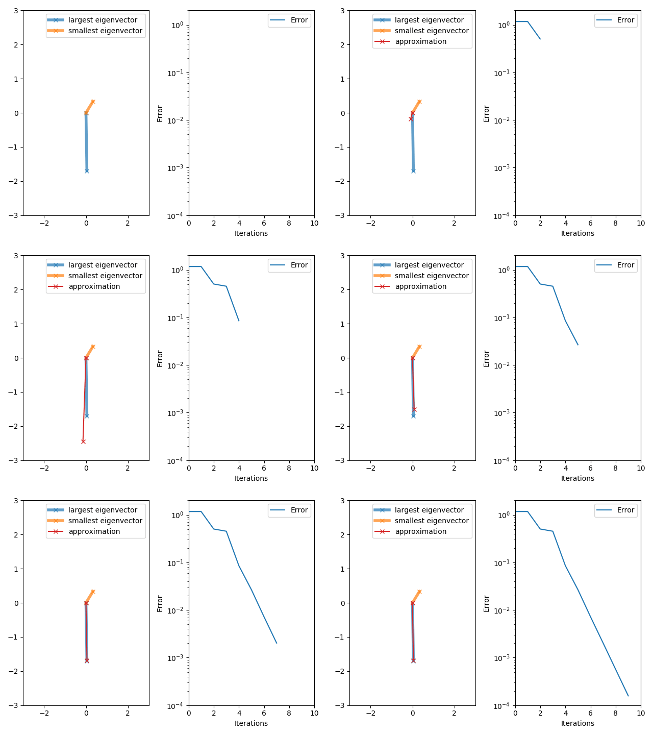
One may compute this with the following algorithm (shown in Python with NumPy):

import numpy as np from numpy import typing as npt def random_vector(dimension: int) -> npt.NDArray[np.float64]: rng = np.random.default_rng() return rng.random(dimension) def power_method( A: npt.NDArray[np.float64], num_iterations: int, ) -> npt.NDArray[np.float64]: if A.shape[0] != A.shape[1]: raise ValueError("A must be a square matrix.") # Choose a random initial vector to reduce the chance # that it is orthogonal to the dominant eigenvector. b_k = random_vector(A.shape[1]) # Normalize the initial vector. b_k /= np.linalg.norm(b_k) for _ in range(num_iterations): # Multiply by the matrix. b_k1 = A @ b_k # Compute the length of the new vector. b_k1_norm = np.linalg.norm(b_k1) # Stop if the new vector is within machine precision of 0. if np.isclose(b_k1_norm, 0.0): raise ValueError("Power method produced the zero vector.") # Normalize the vector for the next iteration. b_k = b_k1 / b_k1_norm # Return the approximate dominant eigenvector. return b_k

The vector $b_{k}$ converges to an associated eigenvector. Ideally, one should use the Rayleigh quotient in order to get the associated eigenvalue.

This algorithm is used to calculate the Google PageRank.

The method can also be used to calculate the spectral radius (the eigenvalue with the largest magnitude, for a square matrix) by computing the Rayleigh quotient

$\rho (A)=\max \left\{\vert \lambda _{1}\vert ,\vert \lambda _{2}\vert ,\ldots ,\vert \lambda _{n}\vert \right\}={\frac {b_{k}^{\top }Ab_{k}}{b_{k}^{\top }b_{k}}}.$

Animation that visualizes the power iteration algorithm on a 2 x 2 matrix. The matrix is depicted by its two eigenvectors. Error is computed as

02Analysis

Let $A$ be decomposed into its Jordan canonical form: $A=VJV^{-1}$ , where the first column of $V$ is an eigenvector of $A$ corresponding to the dominant eigenvalue $\lambda _{1}$ . Since generically, the dominant eigenvalue of $A$ is unique, the first Jordan block of $J$ is the $1\times 1$ matrix $[\lambda _{1}],$ where $\lambda _{1}$ is the largest eigenvalue of $A$ in magnitude. The starting vector $b_{0}$ can be written as a linear combination of the columns of $V$ :

$b_{0}=c_{1}v_{1}+c_{2}v_{2}+\ldots +c_{n}v_{n}.$

By assumption, $b_{0}$ has a nonzero component in the direction of the dominant eigenvector, so $c_{1}\neq 0$ .

The computationally useful recurrence relation for $b_{k+1}$ can be rewritten as:

$b_{k+1}={\frac {Ab_{k}}{\|Ab_{k}\|}}={\frac {A^{k+1}b_{0}}{\|A^{k+1}b_{0}\|}},$

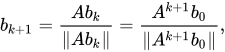
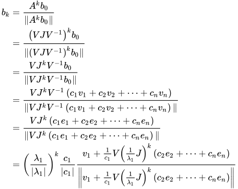
where the expression: ${\frac {A^{k+1}b_{0}}{\|A^{k+1}b_{0}\|}}$ is more amenable to the following analysis:

${\begin{aligned}b_{k}&={\frac {A^{k}b_{0}}{\|A^{k}b_{0}\|}}\\&={\frac {\left(VJV^{-1}\right)^{k}b_{0}}{\|\left(VJV^{-1}\right)^{k}b_{0}\|}}\\&={\frac {VJ^{k}V^{-1}b_{0}}{\|VJ^{k}V^{-1}b_{0}\|}}\\&={\frac {VJ^{k}V^{-1}\left(c_{1}v_{1}+c_{2}v_{2}+\cdots +c_{n}v_{n}\right)}{\|VJ^{k}V^{-1}\left(c_{1}v_{1}+c_{2}v_{2}+\cdots +c_{n}v_{n}\right)\|}}\\&={\frac {VJ^{k}\left(c_{1}e_{1}+c_{2}e_{2}+\cdots +c_{n}e_{n}\right)}{\|VJ^{k}\left(c_{1}e_{1}+c_{2}e_{2}+\cdots +c_{n}e_{n}\right)\|}}\\&=\left({\frac {\lambda _{1}}{|\lambda _{1}|}}\right)^{k}{\frac {c_{1}}{|c_{1}|}}{\frac {v_{1}+{\frac {1}{c_{1}}}V\left({\frac {1}{\lambda _{1}}}J\right)^{k}\left(c_{2}e_{2}+\cdots +c_{n}e_{n}\right)}{\left\|v_{1}+{\frac {1}{c_{1}}}V\left({\frac {1}{\lambda _{1}}}J\right)^{k}\left(c_{2}e_{2}+\cdots +c_{n}e_{n}\right)\right\|}}\end{aligned}}$

The expression above simplifies as $k\to \infty$

$\left({\frac {1}{\lambda _{1}}}J\right)^{k}={\begin{bmatrix}[1]&&&&\\&\left({\frac {1}{\lambda _{1}}}J_{2}\right)^{k}&&&\\&&\ddots &\\&&&\left({\frac {1}{\lambda _{1}}}J_{m}\right)^{k}\\\end{bmatrix}}\rightarrow {\begin{bmatrix}1&&&&\\&0&&&\\&&\ddots &\\&&&0\\\end{bmatrix}}\quad {\text{as}}\quad k\to \infty .$

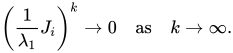
The limit follows from the fact that the eigenvalue of ${\frac {1}{\lambda _{1}}}J_{i}$ is less than 1 in magnitude, so

$\left({\frac {1}{\lambda _{1}}}J_{i}\right)^{k}\to 0\quad {\text{as}}\quad k\to \infty .$

It follows that:

${\frac {1}{c_{1}}}V\left({\frac {1}{\lambda _{1}}}J\right)^{k}\left(c_{2}e_{2}+\cdots +c_{n}e_{n}\right)\to 0\quad {\text{as}}\quad k\to \infty$

Using this fact, $b_{k}$ can be written in a form that emphasizes its relationship with $v_{1}$ when $k$ is large:

${\begin{aligned}b_{k}&=\left({\frac {\lambda _{1}}{|\lambda _{1}|}}\right)^{k}{\frac {c_{1}}{|c_{1}|}}{\frac {v_{1}+{\frac {1}{c_{1}}}V\left({\frac {1}{\lambda _{1}}}J\right)^{k}\left(c_{2}e_{2}+\cdots +c_{n}e_{n}\right)}{\left\|v_{1}+{\frac {1}{c_{1}}}V\left({\frac {1}{\lambda _{1}}}J\right)^{k}\left(c_{2}e_{2}+\cdots +c_{n}e_{n}\right)\right\|}}\\[6pt]&=e^{i\phi _{k}}{\frac {c_{1}}{|c_{1}|}}{\frac {v_{1}}{\|v_{1}\|}}+r_{k}\end{aligned}}$

where $e^{i\phi _{k}}=\left(\lambda _{1}/|\lambda _{1}|\right)^{k}$ and $\|r_{k}\|\to 0$ as $k\to \infty$

The sequence $\left(b_{k}\right)$ is bounded, so it contains a convergent subsequence. Note that the eigenvector corresponding to the dominant eigenvalue is only unique up to a scalar, so although the sequence $\left(b_{k}\right)$ may not converge, $b_{k}$ is nearly an eigenvector of $A$ for large $k$ .

Alternatively, if $A$ is diagonalizable, then the following proof yields the same result:

Let $\lambda _{1},\lambda _{2},\ldots ,\lambda _{m}$ be the $m$ eigenvalues (counted with multiplicity) of $A$ in the order of descending absolute value (equalities allowed), that is $|\lambda _{1}|\geq |\lambda _{2}|\ldots \geq |\lambda _{m}|$ , and let $v_{1},v_{2},\ldots ,v_{m}$ be the corresponding eigenvectors. Suppose that $\lambda _{1}$ is the dominant eigenvalue, so that $|\lambda _{1}|>|\lambda _{j}|$ for all $j>1$ .

The initial vector $b_{0}$ can be written:

$b_{0}=c_{1}v_{1}+c_{2}v_{2}+\cdots +c_{m}v_{m}.$

If $b_{0}$ is chosen randomly (with uniform probability), then $c_{1}\neq 0$ with probability 1. Now,

${\begin{aligned}A^{k}b_{0}&=c_{1}A^{k}v_{1}+c_{2}A^{k}v_{2}+\cdots +c_{m}A^{k}v_{m}\\&=c_{1}\lambda _{1}^{k}v_{1}+c_{2}\lambda _{2}^{k}v_{2}+\cdots +c_{m}\lambda _{m}^{k}v_{m}\\&=c_{1}\lambda _{1}^{k}\left(v_{1}+{\frac {c_{2}}{c_{1}}}\left({\frac {\lambda _{2}}{\lambda _{1}}}\right)^{k}v_{2}+\cdots +{\frac {c_{m}}{c_{1}}}\left({\frac {\lambda _{m}}{\lambda _{1}}}\right)^{k}v_{m}\right)\\&\to c_{1}\lambda _{1}^{k}v_{1}&&\left|{\frac {\lambda _{j}}{\lambda _{1}}}\right|<1{\text{ for }}j>1\end{aligned}}$

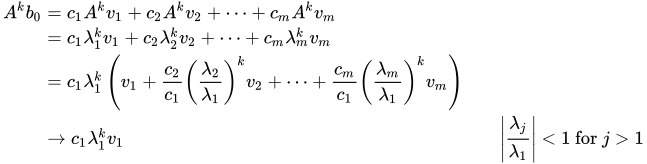
On the other hand:

$b_{k}={\frac {A^{k}b_{0}}{\|A^{k}b_{0}\|}}.$

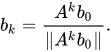
Therefore, $b_{k}$ converges to (a multiple of) the eigenvector $v_{1}$ . The convergence is geometric, with ratio

$\left|{\frac {\lambda _{2}}{\lambda _{1}}}\right|.$

Thus, the method converges slowly if there is an eigenvalue close in magnitude to the dominant eigenvalue.

03Applications

Although the power iteration method approximates only one eigenvalue of a matrix, it remains useful for certain computational problems. For instance, Google uses it to calculate the PageRank of documents in their search engine, and Twitter uses it to show users recommendations of whom to follow. The power iteration method is especially suitable for sparse matrices, such as the web matrix, or as the matrix-free method that does not require storing the coefficient matrix $A$ explicitly, but can instead access a function evaluating matrix-vector products $Ax$ . For non-symmetric matrices that are well-conditioned the power iteration method can outperform more complex Arnoldi iteration. For symmetric matrices, the power iteration method is rarely used, since its convergence speed can be easily increased without sacrificing the small cost per iteration; see, e.g., Lanczos iteration and LOBPCG.

Some of the more advanced eigenvalue algorithms can be understood as variations of the power iteration. For instance, the inverse iteration method applies power iteration to the matrix $A^{-1}$ . Other algorithms look at the whole subspace generated by the vectors $b_{k}$ . This subspace is known as the Krylov subspace. It can be computed by Arnoldi iteration or Lanczos iteration. Gram iteration is a super-linear and deterministic method to compute the largest eigenpair.

Watch videos about Power iterationExplainers and documentaries on YouTube (opens in a new tab)

Sources and credits

This article is adapted from the Wikipedia article “Power iteration”, written by its contributors and licensed under CC BY-SA 4.0. Fathomly has changed the layout, removed citation markers, navigation and maintenance notices, and adjusted punctuation. This adapted version is shared under the same license. For references, see the original article.

Images, from Wikimedia Commons:

Animation of the Power Iteration Algorithm.gif by Alexmath1994, CC BY-SA 4.0

Fathomly is not affiliated with or endorsed by the Wikimedia Foundation. Spotted a problem? Tell us.

Power iteration

01The method

02Analysis

03Applications

Sources and credits

Related topics

Rayleigh quotient iteration

Inverse iteration