Encyclopedia

Polygamma function

Meromorphic function

Wikipedia contributorsAdapted for Fathomly · View authors

3 min read
Source updated August 18, 2025

In mathematics, the polygamma function of order m is a meromorphic function on the complex numbers $\mathbb {C}$ defined as the (m + 1)th derivative of the logarithm of the gamma function:

$\psi ^{(m)}(z):={\frac {\mathrm {d} ^{m}}{\mathrm {d} z^{m}}}\psi (z)={\frac {\mathrm {d} ^{m+1}}{\mathrm {d} z^{m+1}}}\ln \Gamma (z).$

Thus

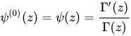
$\psi ^{(0)}(z)=\psi (z)={\frac {\Gamma '(z)}{\Gamma (z)}}$

holds where ψ(z) is the digamma function and Γ(z) is the gamma function. They are holomorphic on $\mathbb {C} \backslash \mathbb {Z} _{\leq 0}$ . At all the nonpositive integers these polygamma functions have a pole of order m + 1. The function ψ⁽¹⁾(z) is sometimes called the trigamma function.

**The logarithm of the gamma function and the first few polygamma functions in the complex plane**

ln Γ(z)	ψ⁽⁰⁾(z)	ψ⁽¹⁾(z)

ψ⁽²⁾(z)	ψ⁽³⁾(z)	ψ⁽⁴⁾(z)

01Integral representation

When m > 0 and Re z > 0, the polygamma function equals

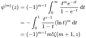
${\begin{aligned}\psi ^{(m)}(z)&=(-1)^{m+1}\int _{0}^{\infty }{\frac {t^{m}e^{-zt}}{1-e^{-t}}}\,\mathrm {d} t\\&=-\int _{0}^{1}{\frac {t^{z-1}}{1-t}}(\ln t)^{m}\,\mathrm {d} t\\&=(-1)^{m+1}m!\zeta (m+1,z)\end{aligned}}$

where $\zeta (s,q)$ is the Hurwitz zeta function.

This expresses the polygamma function as the Laplace transform of ⁠(−1)^m+1 t^m/1 − e^−t⁠. It follows from Bernstein's theorem on monotone functions that, for m > 0 and x real and non-negative, (−1)^m+1 ψ^(m)(x) is a completely monotone function.

Setting m = 0 in the above formula does not give an integral representation of the digamma function. The digamma function has an integral representation, due to Gauss, which is similar to the m = 0 case above but which has an extra term ⁠e^−t/t⁠.

02Recurrence relation

It satisfies the recurrence relation

$\psi ^{(m)}(z+1)=\psi ^{(m)}(z)+{\frac {(-1)^{m}\,m!}{z^{m+1}}}$

which, considered for positive integer argument, leads to a presentation of the sum of reciprocals of the powers of the natural numbers:

${\frac {\psi ^{(m)}(n)}{(-1)^{m+1}\,m!}}=\zeta (1+m)-\sum _{k=1}^{n-1}{\frac {1}{k^{m+1}}}=\sum _{k=n}^{\infty }{\frac {1}{k^{m+1}}}\qquad m\geq 1$

and

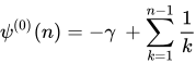
$\psi ^{(0)}(n)=-\gamma \ +\sum _{k=1}^{n-1}{\frac {1}{k}}$

for all $n\in \mathbb {N}$ , where $\gamma$ is the Euler-Mascheroni constant. Like the log-gamma function, the polygamma functions can be generalized from the domain $\mathbb {N}$ uniquely to positive real numbers only due to their recurrence relation and one given function-value, say ψ^(m)(1), except in the case m = 0 where the additional condition of strict monotonicity on $\mathbb {R} ^{+}$ is still needed. This is a trivial consequence of the Bohr-Mollerup theorem for the gamma function where strictly logarithmic convexity on $\mathbb {R} ^{+}$ is demanded additionally. The case m = 0 must be treated differently because ψ⁽⁰⁾ is not normalizable at infinity (the sum of the reciprocals doesn't converge).

03Reflection relation

$(-1)^{m}\psi ^{(m)}(1-z)-\psi ^{(m)}(z)=\pi {\frac {\mathrm {d} ^{m}}{\mathrm {d} z^{m}}}\cot {\pi z}=\pi ^{m+1}{\frac {P_{m}(\cos {\pi z})}{\sin ^{m+1}(\pi z)}}$

where P_m is alternately an odd or even polynomial of degree |m − 1| with integer coefficients and leading coefficient (−1)^m⌈2^{m − 1}⌉. They obey the recursion equation

${\begin{aligned}P_{0}(x)&=x\\P_{m+1}(x)&=-\left((m+1)xP_{m}(x)+\left(1-x^{2}\right)P'_{m}(x)\right).\end{aligned}}$

04Multiplication theorem

The multiplication theorem gives

$k^{m+1}\psi ^{(m)}(kz)=\sum _{n=0}^{k-1}\psi ^{(m)}\left(z+{\frac {n}{k}}\right)\qquad m\geq 1$

and

$k\psi ^{(0)}(kz)=k\ln {k}+\sum _{n=0}^{k-1}\psi ^{(0)}\left(z+{\frac {n}{k}}\right)$

for the digamma function.

05Series representation

The polygamma function has the series representation

$\psi ^{(m)}(z)=(-1)^{m+1}\,m!\sum _{k=0}^{\infty }{\frac {1}{(z+k)^{m+1}}}$

which holds for integer values of m > 0 and any complex z not equal to a negative integer. This representation can be written more compactly in terms of the Hurwitz zeta function as

$\psi ^{(m)}(z)=(-1)^{m+1}\,m!\,\zeta (m+1,z).$

This relation can for example be used to compute the special values

$\psi ^{(2n-1)}\left({\frac {1}{4}}\right)={\frac {4^{2n-1}}{2n}}\left(\pi ^{2n}(2^{2n}-1)|B_{2n}|+2(2n)!\beta (2n)\right);$

$\psi ^{(2n-1)}\left({\frac {3}{4}}\right)={\frac {4^{2n-1}}{2n}}\left(\pi ^{2n}(2^{2n}-1)|B_{2n}|-2(2n)!\beta (2n)\right);$

$\psi ^{(2n)}\left({\frac {1}{4}}\right)=-2^{2n-1}\left(\pi ^{2n+1}|E_{2n}|+2(2n)!(2^{2n+1}-1)\zeta (2n+1)\right);$

$\psi ^{(2n)}\left({\frac {3}{4}}\right)=2^{2n-1}\left(\pi ^{2n+1}|E_{2n}|-2(2n)!(2^{2n+1}-1)\zeta (2n+1)\right).$

Alternately, the Hurwitz zeta can be understood to generalize the polygamma to arbitrary, non-integer order.

One more series may be permitted for the polygamma functions. As given by Schlömilch,

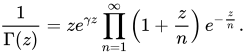
${\frac {1}{\Gamma (z)}}=ze^{\gamma z}\prod _{n=1}^{\infty }\left(1+{\frac {z}{n}}\right)e^{-{\frac {z}{n}}}.$

This is a result of the Weierstrass factorization theorem. Thus, the gamma function may now be defined as:

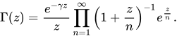
$\Gamma (z)={\frac {e^{-\gamma z}}{z}}\prod _{n=1}^{\infty }\left(1+{\frac {z}{n}}\right)^{-1}e^{\frac {z}{n}}.$

Now, the natural logarithm of the gamma function is easily representable:

$\ln \Gamma (z)=-\gamma z-\ln(z)+\sum _{k=1}^{\infty }\left({\frac {z}{k}}-\ln \left(1+{\frac {z}{k}}\right)\right).$

Finally, we arrive at a summation representation for the polygamma function:

$\psi ^{(n)}(z)={\frac {\mathrm {d} ^{n+1}}{\mathrm {d} z^{n+1}}}\ln \Gamma (z)=-\gamma \delta _{n0}-{\frac {(-1)^{n}n!}{z^{n+1}}}+\sum _{k=1}^{\infty }\left({\frac {1}{k}}\delta _{n0}-{\frac {(-1)^{n}n!}{(k+z)^{n+1}}}\right)$

Where δ_n0 is the Kronecker delta.

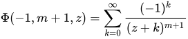
Also the Lerch transcendent

$\Phi (-1,m+1,z)=\sum _{k=0}^{\infty }{\frac {(-1)^{k}}{(z+k)^{m+1}}}$

can be denoted in terms of polygamma function

$\Phi (-1,m+1,z)={\frac {1}{(-2)^{m+1}m!}}\left(\psi ^{(m)}\left({\frac {z}{2}}\right)-\psi ^{(m)}\left({\frac {z+1}{2}}\right)\right)$

06Taylor series

The Taylor series at z = -1 is

$\psi ^{(m)}(z+1)=\sum _{k=0}^{\infty }(-1)^{m+k+1}{\frac {(m+k)!}{k!}}\zeta (m+k+1)z^{k}\qquad m\geq 1$

and

$\psi ^{(0)}(z+1)=-\gamma +\sum _{k=1}^{\infty }(-1)^{k+1}\zeta (k+1)z^{k}$

which converges for |z| < 1. Here, ζ is the Riemann zeta function. This series is easily derived from the corresponding Taylor series for the Hurwitz zeta function. This series may be used to derive a number of rational zeta series.

07Asymptotic expansion

These non-converging series can be used to get quickly an approximation value with a certain numeric at-least-precision for large arguments:

$\psi ^{(m)}(z)\sim (-1)^{m+1}\sum _{k=0}^{\infty }{\frac {(k+m-1)!}{k!}}{\frac {B_{k}}{z^{k+m}}}\qquad m\geq 1$

and

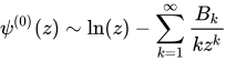
$\psi ^{(0)}(z)\sim \ln(z)-\sum _{k=1}^{\infty }{\frac {B_{k}}{kz^{k}}}$

where we have chosen B₁ = ⁠1/2⁠, i.e. the Bernoulli numbers of the second kind.

08Inequalities

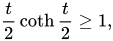
The hyperbolic cotangent satisfies the inequality

${\frac {t}{2}}\operatorname {coth} {\frac {t}{2}}\geq 1,$

and this implies that the function

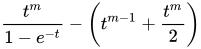
${\frac {t^{m}}{1-e^{-t}}}-\left(t^{m-1}+{\frac {t^{m}}{2}}\right)$

is non-negative for all m ≥ 1 and t ≥ 0. It follows that the Laplace transform of this function is completely monotone. By the integral representation above, we conclude that

$(-1)^{m+1}\psi ^{(m)}(x)-\left({\frac {(m-1)!}{x^{m}}}+{\frac {m!}{2x^{m+1}}}\right)$

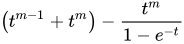
is completely monotone. The convexity inequality e^t ≥ 1 + t implies that

$\left(t^{m-1}+t^{m}\right)-{\frac {t^{m}}{1-e^{-t}}}$

is non-negative for all m ≥ 1 and t ≥ 0, so a similar Laplace transformation argument yields the complete monotonicity of

$\left({\frac {(m-1)!}{x^{m}}}+{\frac {m!}{x^{m+1}}}\right)-(-1)^{m+1}\psi ^{(m)}(x).$

Therefore, for all m ≥ 1 and x > 0,

${\frac {(m-1)!}{x^{m}}}+{\frac {m!}{2x^{m+1}}}\leq (-1)^{m+1}\psi ^{(m)}(x)\leq {\frac {(m-1)!}{x^{m}}}+{\frac {m!}{x^{m+1}}}.$

Since both bounds are strictly positive for $x>0$ , we have:

$\ln \Gamma (x)$ is strictly convex.
For $m=0$ , the digamma function, $\psi (x)=\psi ^{(0)}(x)$ , is strictly monotonic increasing and strictly concave.
For $m$ odd, the polygamma functions, $\psi ^{(1)},\psi ^{(3)},\psi ^{(5)},\ldots$ , are strictly positive, strictly monotonic decreasing and strictly convex.
For $m$ even the polygamma functions, $\psi ^{(2)},\psi ^{(4)},\psi ^{(6)},\ldots$ , are strictly negative, strictly monotonic increasing and strictly concave.

This can be seen in the first plot above.

Trigamma bounds and asymptote

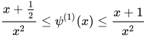
For the case of the trigamma function ( $m=1$ ) the final inequality formula above for $x>0$ , can be rewritten as:

${\frac {x+{\frac {1}{2}}}{x^{2}}}\leq \psi ^{(1)}(x)\leq {\frac {x+1}{x^{2}}}$

so that for $x\gg 1$ : $\psi ^{(1)}(x)\approx {\frac {1}{x}}$ .

Watch videos about Polygamma functionExplainers and documentaries on YouTube (opens in a new tab)

Sources and credits

This article is adapted from the Wikipedia article “Polygamma function”, written by its contributors and licensed under CC BY-SA 4.0. Fathomly has changed the layout, removed citation markers, navigation and maintenance notices, and adjusted punctuation. This adapted version is shared under the same license. For references, see the original article.

Images, from Wikimedia Commons:

Mplwp polygamma03.svg by Geek3, CC BY 3.0
Plot of polygamma function in the complex plane from -2-2i to 2+2i with colors created with Mathematica 13.1.svg by WalkingRadiance, CC BY-SA 4.0
Complex LogGamma.jpg by Jan Homann, Public domain
Complex Polygamma 0.jpg by Jan Homann, Public domain
Complex Polygamma 1.jpg by Jan Homann, Public domain
Complex Polygamma 2.jpg by Jan Homann, Public domain
Complex Polygamma 3.jpg by Jan Homann, Public domain
Complex Polygamma 4.jpg by Jan Homann, Public domain

Fathomly is not affiliated with or endorsed by the Wikimedia Foundation. Spotted a problem? Tell us.