Plug flow
Simple model of fluid flow in a pipe

In fluid mechanics, plug flow is a simple model of the velocity profile of a fluid flowing in a pipe. In plug flow, the velocity of the fluid is assumed to be constant across any cross-section of the pipe perpendicular to the axis of the pipe. The plug flow model assumes there is no boundary layer adjacent to the inner wall of the pipe.
The plug flow model has many practical applications. One example is in the design of chemical reactors. Essentially no back mixing is assumed with "plugs" of fluid passing through the reactor. This results in differential equations that need to be integrated to find the reactor conversion and outlet temperatures. Other simplifications used are perfect radial mixing and a homogeneous bed structure.
An advantage of the plug flow model is that no part of the solution of the problem can be perpetuated "upstream". This allows one to calculate the exact solution to the differential equation knowing only the initial conditions. No further iteration is required. Each "plug" can be solved independently provided the previous plug's state is known.
The flow model in which the velocity profile consists of the fully developed boundary layer is known as pipe flow. In laminar pipe flow, the velocity profile is parabolic.
01Determination
For flows in pipes, if flow is turbulent then the laminar sublayer caused by the pipe wall is so thin that it is negligible. Plug flow will be achieved if the sublayer thickness is much less than the pipe diameter (

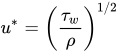

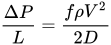

where 


Sources and credits
This article is adapted from the Wikipedia article “Plug flow”, written by its contributors and licensed under CC BY-SA 4.0. Fathomly has changed the layout, removed citation markers, navigation and maintenance notices, and adjusted punctuation. This adapted version is shared under the same license. For references, see the original article.
Images, from Wikimedia Commons:
- Plugflow.jpg by Unknown author, Public domain
Fathomly is not affiliated with or endorsed by the Wikimedia Foundation. Spotted a problem? Tell us.
