Reference articles on history, science, culture and more
Encyclopedia

Directional derivative

Instantaneous rate of change of the function

In multivariable calculus, the directional derivative measures the instantaneous rate at which a function changes along a specified vector through a given point. If the vector is multiplied by a scalar, the corresponding directional derivative is multiplied by the same scalar.

Some elementary texts instead use the phrase "directional derivative in the direction of v" for the rate of change of a function per unit distance in that direction. In that convention the nonzero vector v is first normalized to the unit vector {\hat {\mathbf {v} }}=\mathbf {v} /\|\mathbf {v} \|, where the normalized vector is denoted with a circumflex (hat) symbol: \mathbf {\widehat {}}.

The directional derivative of a scalar function f with respect to a vector v may be denoted by any of the following: {\begin{aligned}\nabla _{\mathbf {v} }{f}(\mathbf {x} )&=f'_{\mathbf {v} }(\mathbf {x} )\\&=D_{\mathbf {v} }f(\mathbf {x} )\\&=Df(\mathbf {x} )(\mathbf {v} )\\&=\partial _{\mathbf {v} }f(\mathbf {x} )\\&={\frac {\partial f(\mathbf {x} )}{\partial \mathbf {v} }}\\&=\mathbf {v} \cdot {\nabla f(\mathbf {x} )}\\&=\mathbf {v} \cdot {\frac {\partial f(\mathbf {x} )}{\partial \mathbf {x} }}.\\\end{aligned}}

It therefore generalizes the notion of a partial derivative, in which the rate of change is taken along one of the curvilinear coordinate curves, all other coordinates being constant. In functional analysis, the analogous notion for functions between topological vector spaces is the Gateaux derivative.

01Definition

The directional derivative of a scalar function f(\mathbf {x} )=f(x_{1},x_{2},\ldots ,x_{n}) along a vector \mathbf {v} =(v_{1},\ldots ,v_{n}) is the function \nabla _{\mathbf {v} }{f} defined by the limit \nabla _{\mathbf {v} }{f}(\mathbf {x} )=\lim _{h\to 0}{\frac {f(\mathbf {x} +h\mathbf {v} )-f(\mathbf {x} )}{h}}=\left.{\frac {\mathrm {d} }{\mathrm {d} t}}f(\mathbf {x} +t\mathbf {v} )\right|_{t=0}.

This definition is valid in a broad range of contexts, for example, where the norm of a vector is defined. In finite dimensions, it does not depend on the choice of norm, since all norms are equivalent. Its applicability extends to functions on finite-dimensional vector spaces without a metric and to differentiable manifolds, such as in general relativity.

For differentiable functions

If the function f is differentiable at x, then the directional derivative exists along any vector v at x, and one has

\nabla _{\mathbf {v} }{f}(\mathbf {x} )=\nabla f(\mathbf {x} )\cdot \mathbf {v}

where the \nabla on the right denotes the gradient and \cdot is the dot product.

It can be derived by using the property that all directional derivatives at a point make up a single tangent plane which can be defined using partial derivatives. This can be used to find a formula for the gradient vector and an alternative formula for the directional derivative, the latter of which can be rewritten as shown above for convenience.

It also follows from defining a path \mathbf {h} (t)=\mathbf {x} +t\mathbf {v} and using the definition of the derivative as a limit along this path to get {\begin{aligned}\nabla _{\mathbf {v} }f(\mathbf {x} )-\nabla f(\mathbf {x} )\cdot \mathbf {v} &=\lim _{t\to 0}{\frac {f(\mathbf {x} +t\mathbf {v} )-f(\mathbf {x} )}{t}}-\nabla f(\mathbf {x} )\cdot \mathbf {v} \\&=\lim _{t\to 0}{\frac {f(\mathbf {x} +t\mathbf {v} )-f(\mathbf {x} )-t\nabla f(\mathbf {x} )\cdot \mathbf {v} }{t}}\\&=0,\end{aligned}} whence \nabla f(\mathbf {x} )\cdot \mathbf {v} =\nabla _{\mathbf {v} }f(\mathbf {x} ).

Using only direction of vector

In a Euclidean space, some authors define the directional derivative to be with respect to an arbitrary nonzero vector v after normalization, thus being independent of its magnitude and depending only on its direction.

This definition gives the rate change of a function f per unit of distance moved in the direction given by v. In this case, one has \nabla _{\hat {\mathbf {v} }}{f}(\mathbf {x} )=\lim _{h\to 0}{\frac {f(\mathbf {x} +h\mathbf {v} )-f(\mathbf {x} )}{h\|v\|}}, or in case f is differentiable at x, \nabla _{\hat {\mathbf {v} }}{f}(\mathbf {x} )=\nabla f(\mathbf {x} )\cdot {\hat {\mathbf {v} }}.

A contour plot of , showing the gradient vector in black, and the unit vector scaled by the directional derivative in the direction of in orange. The gradient vector is longer because the gradient points in the direction of greatest rate of increase of a function.

02Properties

Many of the familiar properties of the ordinary derivative hold for the directional derivative. These include, for any functions f and g defined in a neighborhood of, and differentiable at, p:

  1. sum rule: \nabla _{\mathbf {v} }(f+g)=\nabla _{\mathbf {v} }f+\nabla _{\mathbf {v} }g.
  2. constant factor rule: For any constant c, \nabla _{\mathbf {v} }(cf)=c\nabla _{\mathbf {v} }f.
  3. product rule (or Leibniz's rule): \nabla _{\mathbf {v} }(fg)=g\nabla _{\mathbf {v} }f+f\nabla _{\mathbf {v} }g.
  4. chain rule: If g is differentiable at p and h is differentiable at g(p), then \nabla _{\mathbf {v} }(h\circ g)(\mathbf {p} )=h'(g(\mathbf {p} ))\nabla _{\mathbf {v} }g(\mathbf {p} ).

03In differential geometry

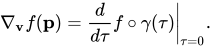
Let M be a differentiable manifold and p a point of M. Suppose that f is a function defined in a neighborhood of p, and differentiable at p. If v is a tangent vector to M at p, then the directional derivative of f along v, denoted variously as df(v) (see Exterior derivative), \nabla _{\mathbf {v} }f(\mathbf {p} ) (see Covariant derivative), L_{\mathbf {v} }f(\mathbf {p} ) (see Lie derivative), or {\mathbf {v} }_{\mathbf {p} }(f) (see Tangent space § Definition via derivations), can be defined as follows. Let γ : [−1, 1] → M be a differentiable curve with γ(0) = p and γ′(0) = v. Then the directional derivative is defined by \nabla _{\mathbf {v} }f(\mathbf {p} )=\left.{\frac {d}{d\tau }}f\circ \gamma (\tau )\right|_{\tau =0}. This definition can be proven independent of the choice of γ, provided γ is selected in the prescribed manner so that γ(0) = p and γ′(0) = v.

The Lie derivative

The Lie derivative of a vector field W^{\mu }(x) along a vector field V^{\mu }(x) is given by the difference of two directional derivatives (with vanishing torsion): {\mathcal {L}}_{V}W^{\mu }=(V\cdot \nabla )W^{\mu }-(W\cdot \nabla )V^{\mu }. In particular, for a scalar field \phi (x), the Lie derivative reduces to the standard directional derivative: {\mathcal {L}}_{V}\phi =(V\cdot \nabla )\phi .

The Riemann tensor

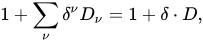
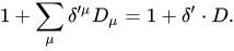
Directional derivatives are often used in introductory derivations of the Riemann curvature tensor. Consider a curved rectangle with an infinitesimal vector \delta along one edge and \delta ' along the other. We translate a covector S along \delta then \delta ' and then subtract the translation along \delta ' and then \delta. Instead of building the directional derivative using partial derivatives, we use the covariant derivative. The translation operator for \delta is thus 1+\sum _{\nu }\delta ^{\nu }D_{\nu }=1+\delta \cdot D, and for \delta ', 1+\sum _{\mu }\delta '^{\mu }D_{\mu }=1+\delta '\cdot D. The difference between the two paths is then (1+\delta '\cdot D)(1+\delta \cdot D)S^{\rho }-(1+\delta \cdot D)(1+\delta '\cdot D)S^{\rho }=\sum _{\mu ,\nu }\delta '^{\mu }\delta ^{\nu }[D_{\mu },D_{\nu }]S_{\rho }. It can be argued that the noncommutativity of the covariant derivatives measures the curvature of the manifold: [D_{\mu },D_{\nu }]S_{\rho }=\pm \sum _{\sigma }R^{\sigma }{}_{\rho \mu \nu }S_{\sigma }, where R is the Riemann curvature tensor and the sign depends on the sign convention of the author.

04In group theory

Translations

In the Poincaré algebra, we can define an infinitesimal translation operator P as \mathbf {P} =i\nabla . (the i ensures that P is a self-adjoint operator) For a finite displacement λ, the unitary Hilbert space representation for translations is U({\boldsymbol {\lambda }})=\exp \left(-i{\boldsymbol {\lambda }}\cdot \mathbf {P} \right). By using the above definition of the infinitesimal translation operator, we see that the finite translation operator is an exponentiated directional derivative: U({\boldsymbol {\lambda }})=\exp \left({\boldsymbol {\lambda }}\cdot \nabla \right). This is a translation operator in the sense that it acts on multivariable functions f(x) as U({\boldsymbol {\lambda }})f(\mathbf {x} )=\exp \left({\boldsymbol {\lambda }}\cdot \nabla \right)f(\mathbf {x} )=f(\mathbf {x} +{\boldsymbol {\lambda }}).

Proof of the last equation

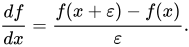
In standard single-variable calculus, the derivative of a smooth function f(x) is defined by (for small ε) {\frac {df}{dx}}={\frac {f(x+\varepsilon )-f(x)}{\varepsilon }}. This can be rearranged to find f(x+ε): f(x+\varepsilon )=f(x)+\varepsilon \,{\frac {df}{dx}}=\left(1+\varepsilon \,{\frac {d}{dx}}\right)f(x). It follows that [1+\varepsilon \,(d/dx)] is a translation operator. This is instantly generalized to multivariable functions f(x) f(\mathbf {x} +{\boldsymbol {\varepsilon }})=\left(1+{\boldsymbol {\varepsilon }}\cdot \nabla \right)f(\mathbf {x} ). Here {\boldsymbol {\varepsilon }}\cdot \nabla is the directional derivative along the infinitesimal displacement ε. We have found the infinitesimal version of the translation operator: U({\boldsymbol {\varepsilon }})=1+{\boldsymbol {\varepsilon }}\cdot \nabla . It is evident that the group multiplication law U(g)U(f)=U(gf) takes the form U(\mathbf {a} )U(\mathbf {b} )=U(\mathbf {a+b} ). So suppose that we take the finite displacement λ and divide it into N parts (N→∞ is implied everywhere), so that λ/N=ε. In other words, {\boldsymbol {\lambda }}=N{\boldsymbol {\varepsilon }}. Then by applying U(ε) N times, we can construct U(λ): [U({\boldsymbol {\varepsilon }})]^{N}=U(N{\boldsymbol {\varepsilon }})=U({\boldsymbol {\lambda }}). We can now plug in our above expression for U(ε): [U({\boldsymbol {\varepsilon }})]^{N}=\left[1+{\boldsymbol {\varepsilon }}\cdot \nabla \right]^{N}=\left[1+{\frac {{\boldsymbol {\lambda }}\cdot \nabla }{N}}\right]^{N}. Using the identity \exp(x)=\left[1+{\frac {x}{N}}\right]^{N}, we have U({\boldsymbol {\lambda }})=\exp \left({\boldsymbol {\lambda }}\cdot \nabla \right). And since U(ε)f(x) = f(x+ε) we have [U({\boldsymbol {\varepsilon }})]^{N}f(\mathbf {x} )=f(\mathbf {x} +N{\boldsymbol {\varepsilon }})=f(\mathbf {x} +{\boldsymbol {\lambda }})=U({\boldsymbol {\lambda }})f(\mathbf {x} )=\exp \left({\boldsymbol {\lambda }}\cdot \nabla \right)f(\mathbf {x} ), Q.E.D.
As a technical note, this procedure is only possible because the translation group forms an Abelian subgroup (Cartan subalgebra) in the Poincaré algebra. In particular, the group multiplication law U(a)U(b) = U(a+b) should not be taken for granted. We also note that Poincaré is a connected Lie group. It is a group of transformations T(ξ) that are described by a continuous set of real parameters \xi ^{a}. The group multiplication law takes the form T({\bar {\xi }})T(\xi )=T(f({\bar {\xi }},\xi )). Taking \xi ^{a}=0 as the coordinates of the identity, we must have f^{a}(\xi ,0)=f^{a}(0,\xi )=\xi ^{a}. The actual operators on the Hilbert space are represented by unitary operators U(T(ξ)). In the above notation we suppressed the T; we now write U(λ) as U(P(λ)). For a small neighborhood around the identity, the power series representation U(T(\xi ))=1+i\sum _{a}\xi ^{a}t_{a}+{\frac {1}{2}}\sum _{b,c}\xi ^{b}\xi ^{c}t_{bc}+\cdots is quite good. Suppose that U(T(ξ)) form a non-projective representation, i.e., U(T({\bar {\xi }}))U(T(\xi ))=U(T(f({\bar {\xi }},\xi ))). The expansion of f to second power is f^{a}({\bar {\xi }},\xi )=\xi ^{a}+{\bar {\xi }}^{a}+\sum _{b,c}f^{abc}{\bar {\xi }}^{b}\xi ^{c}. After expanding the representation multiplication equation and equating coefficients, we have the nontrivial condition t_{bc}=-t_{b}t_{c}-i\sum _{a}f^{abc}t_{a}. Since t_{ab} is by definition symmetric in its indices, we have the standard Lie algebra commutator: [t_{b},t_{c}]=i\sum _{a}(-f^{abc}+f^{acb})t_{a}=i\sum _{a}C^{abc}t_{a}, with C the structure constant. The generators for translations are partial derivative operators, which commute: \left[{\frac {\partial }{\partial x^{b}}},{\frac {\partial }{\partial x^{c}}}\right]=0. This implies that the structure constants vanish and thus the quadratic coefficients in the f expansion vanish as well. This means that f is simply additive: f_{\text{abelian}}^{a}({\bar {\xi }},\xi )=\xi ^{a}+{\bar {\xi }}^{a}, and thus for abelian groups, U(T({\bar {\xi }}))U(T(\xi ))=U(T({\bar {\xi }}+\xi )). Q.E.D.

Rotations

The rotation operator also contains a directional derivative. The rotation operator for an angle θ, i.e. by an amount θ = |θ| about an axis parallel to {\hat {\theta }}={\boldsymbol {\theta }}/\theta is U(R(\mathbf {\theta } ))=\exp(-i\mathbf {\theta } \cdot \mathbf {L} ). Here L is the vector operator that generates SO(3): \mathbf {L} ={\begin{pmatrix}0&0&0\\0&0&1\\0&-1&0\end{pmatrix}}\mathbf {i} +{\begin{pmatrix}0&0&-1\\0&0&0\\1&0&0\end{pmatrix}}\mathbf {j} +{\begin{pmatrix}0&1&0\\-1&0&0\\0&0&0\end{pmatrix}}\mathbf {k} . It may be shown geometrically that an infinitesimal right-handed rotation changes the position vector x by \mathbf {x} \rightarrow \mathbf {x} -\delta {\boldsymbol {\theta }}\times \mathbf {x} . So we would expect under infinitesimal rotation: U(R(\delta {\boldsymbol {\theta }}))f(\mathbf {x} )=f(\mathbf {x} -\delta {\boldsymbol {\theta }}\times \mathbf {x} )=f(\mathbf {x} )-(\delta {\boldsymbol {\theta }}\times \mathbf {x} )\cdot \nabla f. It follows that U(R(\delta \mathbf {\theta } ))=1-(\delta \mathbf {\theta } \times \mathbf {x} )\cdot \nabla . Following the same exponentiation procedure as above, we arrive at the rotation operator in the position basis, which is an exponentiated directional derivative: U(R(\mathbf {\theta } ))=\exp(-(\mathbf {\theta } \times \mathbf {x} )\cdot \nabla ).

The angle α between the tangent A and the horizontal will be maximum if the cutting plane contains the direction of the gradient A.

05Normal derivative

A normal derivative is a directional derivative taken in the direction normal (that is, orthogonal) to some surface in space, or more generally along a normal vector field orthogonal to some hypersurface. See for example Neumann boundary condition. If the normal direction is denoted by \mathbf {n}, then the normal derivative of a function f is sometimes denoted as {\textstyle {\frac {\partial f}{\partial \mathbf {n} }}. In other notations, {\frac {\partial f}{\partial \mathbf {n} }}=\nabla f(\mathbf {x} )\cdot \mathbf {n} =\nabla _{\mathbf {n} }{f}(\mathbf {x} )={\frac {\partial f}{\partial \mathbf {x} }}\cdot \mathbf {n} =Df(\mathbf {x} )[\mathbf {n} ].

06In the continuum mechanics of solids

Several important results in continuum mechanics require the derivatives of vectors with respect to vectors and of tensors with respect to vectors and tensors. The directional derivative provides a systematic way of finding these derivatives.

The definitions of directional derivatives for various situations are given below. It is assumed that the functions are sufficiently smooth that derivatives can be taken.

Derivatives of scalar valued functions of vectors

Let f(v) be a real valued function of the vector v. Then the derivative of f(v) with respect to v (or at v) is the vector defined through its dot product with any vector u being

{\frac {\partial f}{\partial \mathbf {v} }}\cdot \mathbf {u} =Df(\mathbf {v} )[\mathbf {u} ]=\left[{\frac {d}{d\alpha }}~f(\mathbf {v} +\alpha ~\mathbf {u} )\right]_{\alpha =0}

for all vectors u. The above dot product yields a scalar, and if u is a unit vector gives the directional derivative of f at v, in the u direction.

Properties:

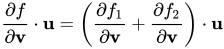
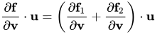
  1. If f(\mathbf {v} )=f_{1}(\mathbf {v} )+f_{2}(\mathbf {v} ) then {\frac {\partial f}{\partial \mathbf {v} }}\cdot \mathbf {u} =\left({\frac {\partial f_{1}}{\partial \mathbf {v} }}+{\frac {\partial f_{2}}{\partial \mathbf {v} }}\right)\cdot \mathbf {u}
  2. If f(\mathbf {v} )=f_{1}(\mathbf {v} )~f_{2}(\mathbf {v} ) then {\frac {\partial f}{\partial \mathbf {v} }}\cdot \mathbf {u} =\left({\frac {\partial f_{1}}{\partial \mathbf {v} }}\cdot \mathbf {u} \right)~f_{2}(\mathbf {v} )+f_{1}(\mathbf {v} )~\left({\frac {\partial f_{2}}{\partial \mathbf {v} }}\cdot \mathbf {u} \right)
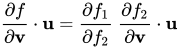
  3. If f(\mathbf {v} )=f_{1}(f_{2}(\mathbf {v} )) then {\frac {\partial f}{\partial \mathbf {v} }}\cdot \mathbf {u} ={\frac {\partial f_{1}}{\partial f_{2}}}~{\frac {\partial f_{2}}{\partial \mathbf {v} }}\cdot \mathbf {u}

Derivatives of vector valued functions of vectors

Let f(v) be a vector valued function of the vector v. Then the derivative of f(v) with respect to v (or at v) is the second order tensor defined through its dot product with any vector u being

{\frac {\partial \mathbf {f} }{\partial \mathbf {v} }}\cdot \mathbf {u} =D\mathbf {f} (\mathbf {v} )[\mathbf {u} ]=\left[{\frac {d}{d\alpha }}~\mathbf {f} (\mathbf {v} +\alpha ~\mathbf {u} )\right]_{\alpha =0}

for all vectors u. The above dot product yields a vector, and if u is a unit vector gives the direction derivative of f at v, in the directional u.

Properties:

  1. If \mathbf {f} (\mathbf {v} )=\mathbf {f} _{1}(\mathbf {v} )+\mathbf {f} _{2}(\mathbf {v} ) then {\frac {\partial \mathbf {f} }{\partial \mathbf {v} }}\cdot \mathbf {u} =\left({\frac {\partial \mathbf {f} _{1}}{\partial \mathbf {v} }}+{\frac {\partial \mathbf {f} _{2}}{\partial \mathbf {v} }}\right)\cdot \mathbf {u}
  2. If \mathbf {f} (\mathbf {v} )=\mathbf {f} _{1}(\mathbf {v} )\times \mathbf {f} _{2}(\mathbf {v} ) then {\frac {\partial \mathbf {f} }{\partial \mathbf {v} }}\cdot \mathbf {u} =\left({\frac {\partial \mathbf {f} _{1}}{\partial \mathbf {v} }}\cdot \mathbf {u} \right)\times \mathbf {f} _{2}(\mathbf {v} )+\mathbf {f} _{1}(\mathbf {v} )\times \left({\frac {\partial \mathbf {f} _{2}}{\partial \mathbf {v} }}\cdot \mathbf {u} \right)
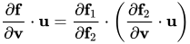
  3. If \mathbf {f} (\mathbf {v} )=\mathbf {f} _{1}(\mathbf {f} _{2}(\mathbf {v} )) then {\frac {\partial \mathbf {f} }{\partial \mathbf {v} }}\cdot \mathbf {u} ={\frac {\partial \mathbf {f} _{1}}{\partial \mathbf {f} _{2}}}\cdot \left({\frac {\partial \mathbf {f} _{2}}{\partial \mathbf {v} }}\cdot \mathbf {u} \right)

Derivatives of scalar valued functions of second-order tensors

Let f({\boldsymbol {S}}) be a real valued function of the second order tensor {\boldsymbol {S}}. Then the derivative of f({\boldsymbol {S}}) with respect to {\boldsymbol {S}} (or at {\boldsymbol {S}}) in the direction {\boldsymbol {T}} is the second order tensor defined as {\frac {\partial f}{\partial {\boldsymbol {S}}}}:{\boldsymbol {T}}=Df({\boldsymbol {S}})[{\boldsymbol {T}}]=\left[{\frac {d}{d\alpha }}~f({\boldsymbol {S}}+\alpha ~{\boldsymbol {T}})\right]_{\alpha =0} for all second order tensors {\boldsymbol {T}}.

Properties:

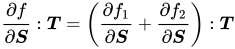
  1. If f({\boldsymbol {S}})=f_{1}({\boldsymbol {S}})+f_{2}({\boldsymbol {S}}) then {\frac {\partial f}{\partial {\boldsymbol {S}}}}:{\boldsymbol {T}}=\left({\frac {\partial f_{1}}{\partial {\boldsymbol {S}}}}+{\frac {\partial f_{2}}{\partial {\boldsymbol {S}}}}\right):{\boldsymbol {T}}
  2. If f({\boldsymbol {S}})=f_{1}({\boldsymbol {S}})~f_{2}({\boldsymbol {S}}) then {\frac {\partial f}{\partial {\boldsymbol {S}}}}:{\boldsymbol {T}}=\left({\frac {\partial f_{1}}{\partial {\boldsymbol {S}}}}:{\boldsymbol {T}}\right)~f_{2}({\boldsymbol {S}})+f_{1}({\boldsymbol {S}})~\left({\frac {\partial f_{2}}{\partial {\boldsymbol {S}}}}:{\boldsymbol {T}}\right)
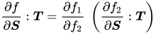
  3. If f({\boldsymbol {S}})=f_{1}(f_{2}({\boldsymbol {S}})) then {\frac {\partial f}{\partial {\boldsymbol {S}}}}:{\boldsymbol {T}}={\frac {\partial f_{1}}{\partial f_{2}}}~\left({\frac {\partial f_{2}}{\partial {\boldsymbol {S}}}}:{\boldsymbol {T}}\right)

Derivatives of tensor valued functions of second-order tensors

Let {\boldsymbol {F}}({\boldsymbol {S}}) be a second order tensor valued function of the second order tensor {\boldsymbol {S}}. Then the derivative of {\boldsymbol {F}}({\boldsymbol {S}}) with respect to {\boldsymbol {S}} (or at {\boldsymbol {S}}) in the direction {\boldsymbol {T}} is the fourth order tensor defined as {\frac {\partial {\boldsymbol {F}}}{\partial {\boldsymbol {S}}}}:{\boldsymbol {T}}=D{\boldsymbol {F}}({\boldsymbol {S}})[{\boldsymbol {T}}]=\left[{\frac {d}{d\alpha }}~{\boldsymbol {F}}({\boldsymbol {S}}+\alpha ~{\boldsymbol {T}})\right]_{\alpha =0} for all second order tensors {\boldsymbol {T}}.

Properties:

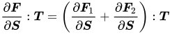
  1. If {\boldsymbol {F}}({\boldsymbol {S}})={\boldsymbol {F}}_{1}({\boldsymbol {S}})+{\boldsymbol {F}}_{2}({\boldsymbol {S}}) then {\frac {\partial {\boldsymbol {F}}}{\partial {\boldsymbol {S}}}}:{\boldsymbol {T}}=\left({\frac {\partial {\boldsymbol {F}}_{1}}{\partial {\boldsymbol {S}}}}+{\frac {\partial {\boldsymbol {F}}_{2}}{\partial {\boldsymbol {S}}}}\right):{\boldsymbol {T}}
  2. If {\boldsymbol {F}}({\boldsymbol {S}})={\boldsymbol {F}}_{1}({\boldsymbol {S}})\cdot {\boldsymbol {F}}_{2}({\boldsymbol {S}}) then {\frac {\partial {\boldsymbol {F}}}{\partial {\boldsymbol {S}}}}:{\boldsymbol {T}}=\left({\frac {\partial {\boldsymbol {F}}_{1}}{\partial {\boldsymbol {S}}}}:{\boldsymbol {T}}\right)\cdot {\boldsymbol {F}}_{2}({\boldsymbol {S}})+{\boldsymbol {F}}_{1}({\boldsymbol {S}})\cdot \left({\frac {\partial {\boldsymbol {F}}_{2}}{\partial {\boldsymbol {S}}}}:{\boldsymbol {T}}\right)
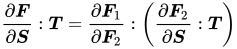
  3. If {\boldsymbol {F}}({\boldsymbol {S}})={\boldsymbol {F}}_{1}({\boldsymbol {F}}_{2}({\boldsymbol {S}})) then {\frac {\partial {\boldsymbol {F}}}{\partial {\boldsymbol {S}}}}:{\boldsymbol {T}}={\frac {\partial {\boldsymbol {F}}_{1}}{\partial {\boldsymbol {F}}_{2}}}:\left({\frac {\partial {\boldsymbol {F}}_{2}}{\partial {\boldsymbol {S}}}}:{\boldsymbol {T}}\right)
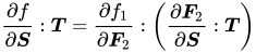
  4. If f({\boldsymbol {S}})=f_{1}({\boldsymbol {F}}_{2}({\boldsymbol {S}})) then {\frac {\partial f}{\partial {\boldsymbol {S}}}}:{\boldsymbol {T}}={\frac {\partial f_{1}}{\partial {\boldsymbol {F}}_{2}}}:\left({\frac {\partial {\boldsymbol {F}}_{2}}{\partial {\boldsymbol {S}}}}:{\boldsymbol {T}}\right)
Watch videos about Directional derivativeExplainers and documentaries on YouTube (opens in a new tab)

Sources and credits

This article is adapted from the Wikipedia article Directional derivative, written by its contributors and licensed under CC BY-SA 4.0. Fathomly has changed the layout, removed citation markers, navigation and maintenance notices, and adjusted punctuation. This adapted version is shared under the same license. For references, see the original article.

Images, from Wikimedia Commons:

Fathomly is not affiliated with or endorsed by the Wikimedia Foundation. Spotted a problem? Tell us.