Shortest path problem
Computational problem of graph theory

In graph theory, the shortest path problem is the problem of finding a path between two vertices (or nodes) in a graph such that the sum of the weights of its constituent edges is minimized.
The problem of finding the shortest path between two intersections on a road map may be modeled as a special case of the shortest path problem in graphs, where the vertices correspond to intersections and the edges correspond to road segments, each weighted by the length or distance of each segment.
01Definition
The shortest path problem can be defined for graphs whether undirected, directed, or mixed. The definition for undirected graphs states that every edge can be traversed in either direction. Directed graphs require that consecutive vertices be connected by an appropriate directed edge.
Two vertices are adjacent when they are both incident to a common edge. A path in an undirected graph is a sequence of vertices 


Let 





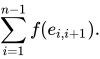

The problem is also sometimes called the single-pair shortest path problem, to distinguish it from the following variations:
- The single-source shortest path problem, in which we have to find shortest paths from a source vertex v to all other vertices in the graph.
- The single-destination shortest path problem, in which we have to find shortest paths from all vertices in the directed graph to a single destination vertex v. This can be reduced to the single-source shortest path problem by reversing the arcs in the directed graph.
- The all-pairs shortest path problem, in which we have to find shortest paths between every pair of vertices v, v' in the graph.
These generalizations have significantly more efficient algorithms than the simplistic approach of running a single-pair shortest path algorithm on all relevant pairs of vertices.
02Algorithms
Several well-known algorithms exist for solving this problem and its variants.
- Dijkstra's algorithm solves the single-source shortest path problem with only non-negative edge weights.
- Bellman-Ford algorithm solves the single-source problem if edge weights may be negative.
- A* search algorithm solves for single-pair shortest path using heuristics to try to speed up the search.
- Floyd-Warshall algorithm solves all pairs shortest paths.
- Johnson's algorithm solves all pairs shortest paths, and may be faster than Floyd-Warshall on sparse graphs.
- Viterbi algorithm solves the shortest stochastic path problem with an additional probabilistic weight on each node.
Additional algorithms and associated evaluations may be found in Cherkassky, Goldberg & Radzik (1996).
03Single-source shortest paths
Undirected graphs
| Weights | Time complexity | Author |
|---|---|---|
 + + |  | Dijkstra 1959 |
| + |  | Johnson 1977 (binary heap) |
| + |  | Fredman & Tarjan 1984 (Fibonacci heap) |
 |  | Thorup 1999 (requires constant-time multiplication) |
| + |  | Duan et al. 2023 |
Unweighted graphs
| Algorithm | Time complexity | Author |
|---|---|---|
| Breadth-first search |  |
Directed acyclic graphs
An algorithm using topological sorting can solve the single-source shortest path problem in time Θ(E + V) in arbitrarily-weighted directed acyclic graphs.
Directed graphs with nonnegative weights
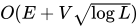
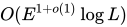
The following table is taken from Schrijver (2004), with some corrections and additions. A green background indicates an asymptotically best bound in the table; L is the maximum length (or weight) among all edges, assuming integer edge weights.
| Weights | Algorithm | Time complexity | Author |
|---|---|---|---|
|  | Ford 1956 | |
| Bellman-Ford algorithm |  | Shimbel 1955, Bellman 1958, Moore 1959 |
|  | Dantzig 1960 | |
| Dijkstra's algorithm with list | | Leyzorek et al. 1957, Dijkstra 1959, Minty (see Pollack & Wiebenson 1960), Whiting & Hillier 1960 |
| Dijkstra's algorithm with binary heap | | Johnson 1977 |
| Dijkstra's algorithm with Fibonacci heap | | Fredman & Tarjan 1984, Fredman & Tarjan 1987 |
| Quantum Dijkstra algorithm with adjacency list | 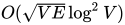 | Dürr et al. 2006 |
|
Dijkstra's-Bellman-Ford hybrid with a divide-and-conquer frontier reduction |  |
Duan et al. 2025 |
| Dial's algorithm (Dijkstra's algorithm using a bucket queue with L buckets) |  | Dial 1969 |
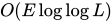 | Johnson 1981, Karlsson & Poblete 1983 | ||
| Gabow's algorithm | 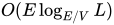 | Gabow 1983, Gabow 1985 | |
 | Ahuja et al. 1990 | ||
| Thorup |  | Thorup 2004 |
Directed graphs with arbitrary weights without negative cycles
| Weights | Algorithm | Time complexity | Author |
|---|---|---|---|
| | Ford 1956 | |
| Bellman-Ford algorithm | | Shimbel 1955, Bellman 1958, Moore 1959 |
| Johnson-Dijkstra with binary heap |  | Johnson 1977 |
| Johnson-Dijkstra with Fibonacci heap | | Fredman & Tarjan 1984, Fredman & Tarjan 1987, adapted after Johnson 1977 |
 | Johnson's technique applied to Dial's algorithm | 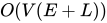 | Dial 1969, adapted after Johnson 1977 |
|
Interior-point method with Laplacian solver |  |
Cohen et al. 2017 |
|
Interior-point method with  flow solver flow solver |
 |
Axiotis, Mądry & Vladu 2020 |
|
Robust interior-point method with sketching |  |
van den Brand et al. 2020 |
|
 interior-point method with dynamic min-ratio cycle data structure interior-point method with dynamic min-ratio cycle data structure |
 |
Chen et al. 2022 |
|
Based on low-diameter decomposition |  |
Bernstein, Nanongkai & Wulff-Nilsen 2022 |
|
Hop-limited shortest paths |  |
Fineman 2024 |
|
Steiner-Tree Gadgets |  |
Khanna & Song 2026 |
Directed graphs with arbitrary weights with negative cycles
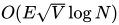
Finds a negative cycle or calculates distances to all vertices.
| Weights | Algorithm | Time complexity | Author |
|---|---|---|---|
|  | Andrew V. Goldberg |
Planar graphs with nonnegative weights
| Weights | Algorithm | Time complexity | Author |
|---|---|---|---|
 |  | Henzinger et al. 1997 |
04Applications
Network flows are a fundamental concept in graph theory and operations research, often used to model problems involving the transportation of goods, liquids, or information through a network. A network flow problem typically involves a directed graph where each edge represents a pipe, wire, or road, and each edge has a capacity, which is the maximum amount that can flow through it. The goal is to find a feasible flow that maximizes the flow from a source node to a sink node.
Shortest Path Problems can be used to solve certain network flow problems, particularly when dealing with single-source, single-sink networks. In these scenarios, we can transform the network flow problem into a series of shortest path problems.
Transformation Steps
- Create a Residual Graph:
- For each edge (u, v) in the original graph, create two edges in the residual graph:
- (u, v) with capacity c(u, v)
- (v, u) with capacity 0
- The residual graph represents the remaining capacity available in the network.
- For each edge (u, v) in the original graph, create two edges in the residual graph:
- Find the Shortest Path:
- Use a shortest path algorithm (e.g., Dijkstra's algorithm, Bellman-Ford algorithm) to find the shortest path from the source node to the sink node in the residual graph.
- Augment the Flow:
- Find the minimum capacity along the shortest path.
- Increase the flow on the edges of the shortest path by this minimum capacity.
- Decrease the capacity of the edges in the forward direction and increase the capacity of the edges in the backward direction.
- Update the Residual Graph:
- Update the residual graph based on the augmented flow.
- Repeat:
- Repeat steps 2-4 until no more paths can be found from the source to the sink.
05All-pairs shortest paths
The all-pairs shortest path problem finds the shortest paths between every pair of vertices v, v' in the graph. The all-pairs shortest paths problem for unweighted directed graphs was introduced by Shimbel (1953), who observed that it could be solved by a linear number of matrix multiplications that takes a total time of O(V4).
Undirected graph
| Weights | Time complexity | Algorithm |
|---|---|---|
| + |  | Floyd-Warshall algorithm |
 |  | Seidel's algorithm (expected running time using fast matrix multiplication algorithms) |
| 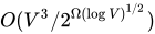 | Williams 2014 |
| + |  | Pettie & Ramachandran 2002 |
|  | Thorup 1999 applied to every vertex (requires constant-time multiplication). |
Directed graph
| Weights | Time complexity | Algorithm |
|---|---|---|
| (no negative cycles) | | Floyd-Warshall algorithm |
| | Williams 2014 |
| (no negative cycles) | 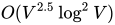 | Quantum search |
| (no negative cycles) |  | Johnson-Dijkstra |
| (no negative cycles) |  | Pettie 2004 |
|
| Hagerup 2000 |
06Applications
Shortest path algorithms are applied to automatically find directions between physical locations, such as driving directions on web mapping websites like MapQuest or Google Maps. For this application fast specialized algorithms are available.
If one represents a nondeterministic abstract machine as a graph where vertices describe states and edges describe possible transitions, shortest path algorithms can be used to find an optimal sequence of choices to reach a certain goal state, or to establish lower bounds on the time needed to reach a given state. For example, if vertices represent the states of a puzzle like a Rubik's Cube and each directed edge corresponds to a single move or turn, shortest path algorithms can be used to find a solution that uses the minimum possible number of moves.
In a networking or telecommunications mindset, this shortest path problem is sometimes called the min-delay path problem and usually tied with a widest path problem. For example, the algorithm may seek the shortest (min-delay) widest path, or widest shortest (min-delay) path.
A more lighthearted application is the games of "six degrees of separation" that try to find the shortest path in graphs like movie stars appearing in the same film.
Other applications, often studied in operations research, include plant and facility layout, robotics, transportation, and VLSI design.
Road networks
A road network can be considered as a graph with positive weights. The nodes represent road junctions and each edge of the graph is associated with a road segment between two junctions. The weight of an edge may correspond to the length of the associated road segment, the time needed to traverse the segment, or the cost of traversing the segment. Using directed edges it is also possible to model one-way streets. Such graphs are special in the sense that some edges are more important than others for long-distance travel (e.g. highways). This property has been formalized using the notion of highway dimension. There are a great number of algorithms that exploit this property and are therefore able to compute the shortest path a lot quicker than would be possible on general graphs.
All of these algorithms work in two phases. In the first phase, the graph is preprocessed without knowing the source or target node. The second phase is the query phase. In this phase, source and target node are known. The idea is that the road network is static, so the preprocessing phase can be done once and used for a large number of queries on the same road network.
The algorithm with the fastest known query time is called hub labeling and is able to compute shortest path on the road networks of Europe or the US in a fraction of a microsecond. Other techniques that have been used are:
- ALT (A* search, landmarks, and triangle inequality)
- Arc flags
- Contraction hierarchies
- Transit node routing
- Reach-based pruning
- Labeling
- Hub labels
07Related problems
For shortest path problems in computational geometry, see Euclidean shortest path.
The shortest multiple disconnected path is a representation of the primitive path network within the framework of Reptation theory. The widest path problem seeks a path so that the minimum label of any edge is as large as possible.
Other related problems may be classified into the following categories.
Paths with constraints
Unlike the shortest path problem, which can be solved in polynomial time in graphs without negative cycles, shortest path problems which include additional constraints on the desired solution path are called Constrained Shortest Path First, and are harder to solve. One example is the constrained shortest path problem, which attempts to minimize the total cost of the path while at the same time maintaining another metric below a given threshold. This makes the problem NP-complete (such problems are not believed to be efficiently solvable for large sets of data, see P = NP problem). Another NP-complete example requires a specific set of vertices to be included in the path, which makes the problem similar to the Traveling Salesman Problem (TSP). The TSP is the problem of finding the shortest path that goes through every vertex exactly once, and returns to the start. The problem of finding the longest path in a graph is also NP-complete.
Partial observability
The Canadian traveller problem and the stochastic shortest path problem are generalizations where either the graph is not completely known to the mover, changes over time, or where actions (traversals) are probabilistic.
Strategic shortest paths
Sometimes, the edges in a graph have personalities: each edge has its own selfish interest. An example is a communication network, in which each edge is a computer that possibly belongs to a different person. Different computers have different transmission speeds, so every edge in the network has a numeric weight equal to the number of milliseconds it takes to transmit a message. Our goal is to send a message between two points in the network in the shortest time possible. If we know the transmission-time of each computer (the weight of each edge), then we can use a standard shortest-paths algorithm. If we do not know the transmission times, then we have to ask each computer to tell us its transmission-time. But, the computers may be selfish: a computer might tell us that its transmission time is very long, so that we will not bother it with our messages. A possible solution to this problem is to use a variant of the VCG mechanism, which gives the computers an incentive to reveal their true weights.
Negative cycle detection
In some cases, the main goal is not to find the shortest path, but only to detect if the graph contains a negative cycle. Some shortest-paths algorithms can be used for this purpose:
- The Bellman-Ford algorithm can be used to detect a negative cycle in time
.
- Cherkassky and Goldberg survey several other algorithms for negative cycle detection.
08General algebraic framework on semirings: the algebraic path problem
Many problems can be framed as a form of the shortest path for some suitably substituted notions of addition along a path and taking the minimum. The general approach to these is to consider the two operations to be those of a semiring. Semiring multiplication is done along the path, and the addition is between paths. This general framework is known as the algebraic path problem.
Most of the classic shortest-path algorithms (and new ones) can be formulated as solving linear systems over such algebraic structures.
More recently, an even more general framework for solving these (and much less obviously related problems) has been developed under the banner of valuation algebras.
09Shortest path in stochastic time-dependent networks
In real-life, a transportation network is usually stochastic and time-dependent. The travel duration on a road segment depends on many factors such as the amount of traffic (origin-destination matrix), road work, weather, accidents and vehicle breakdowns. A more realistic model of such a road network is a stochastic time-dependent (STD) network.
There is no accepted definition of optimal path under uncertainty (that is, in stochastic road networks). It is a controversial subject, despite considerable progress during the past decade. One common definition is a path with the minimum expected travel time. The main advantage of this approach is that it can make use of efficient shortest path algorithms for deterministic networks. However, the resulting optimal path may not be reliable, because this approach fails to address travel time variability.
To tackle this issue, some researchers use travel duration distribution instead of its expected value. So, they find the probability distribution of total travel duration using different optimization methods such as dynamic programming and Dijkstra's algorithm . These methods use stochastic optimization, specifically stochastic dynamic programming to find the shortest path in networks with probabilistic arc length. The terms travel time reliability and travel time variability are used as opposites in the transportation research literature: the higher the variability, the lower the reliability of predictions.
To account for variability, researchers have suggested two alternative definitions for an optimal path under uncertainty. The most reliable path is one that maximizes the probability of arriving on time given a travel time budget. An α-reliable path is one that minimizes the travel time budget required to arrive on time with a given probability.
10Restricted shortest path
The Restricted Shortest Path problem (RSP) is a variant of the shortest path problem in which there are two optimization criteria. We are given a directed graph in which every edge e has a nonnegative integer cost ce, and a nonnegative integer delay de, two designated vertices s and t, and a nonnegative integer delay budget B. The goal is to find an s--t path of minimum total cost, among the paths whose total delay is at most B. RSP is NP-hard: it appears in the book of Garey and Johnson as problem ND30, "Shortest weight-constrained path". It has an FPTAS due to Hassin, later simplified and improved by Lorenz and Raz.
Several generalizations of this problem are known:
- In resource constrained shortest path (RCSP), each edge can consume several resources (rather than just time). Each resource r has an independent budget Br. Each edge e consumes de,r of each resource r. The goal is to find an s--t path of minimum total cost, among the paths that satisfy the resource constraint for each resource.
- In the shared-multi-CSP problem, there can be several source-target pairs (sj,tj), for j=1,2,.. Here, the goal is to find a path for each source-target pair, with a minimum total cost, subject to the total delay being at most the delay budget.
- Fractional RSP is a linear programming relaxation of RSP. Handler and Zang introduced it and gave a combinatorial algorithm for solving it (in the case of one resource). Mehlhorn and Ziegelmann proved that, in the case of one resource, the combinatorial algorithm runs in polytime, O(log (n C D)), where n is the number of nodes, the costs are integers in 0..C, and the delays are integers in 0..D. For many resources the runtime of the combinatorial algorithm remains open, but the LP can be solved in weakly polynomial time using the ellipsoid method.
Sources and credits
This article is adapted from the Wikipedia article “Shortest path problem”, written by its contributors and licensed under CC BY-SA 4.0. Fathomly has changed the layout, removed citation markers, navigation and maintenance notices, and adjusted punctuation. This adapted version is shared under the same license. For references, see the original article.
Images, from Wikimedia Commons:
- Shortest path with direct weights.svg by Artyom Kalinin, CC BY-SA 3.0
Fathomly is not affiliated with or endorsed by the Wikimedia Foundation. Spotted a problem? Tell us.

