Multivariate probit model
In statistics and econometrics, the multivariate probit model is a generalization of the probit model used to estimate several correlated binary outcomes jointly. For example, if it is believed that the decisions of sending at least one child to public school and that of voting in favor of a school budget are correlated (both decisions are binary), then the multivariate probit model would be appropriate for jointly predicting these two choices on an individual-specific basis. J.R. Ashford and R.R. Sowden initially proposed an approach for multivariate probit analysis. Siddhartha Chib and Edward Greenberg extended this idea and also proposed simulation-based inference methods for the multivariate probit model which simplified and generalized parameter estimation.
01Example: bivariate probit
In the ordinary probit model, there is only one binary dependent variable 


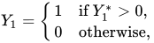
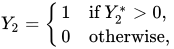
with
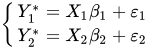
and

Fitting the bivariate probit model involves estimating the values of 

![{\begin{aligned}L(\beta _{1},\beta _{2})={\Big (}\prod &P(Y_{1}=1,Y_{2}=1\mid \beta _{1},\beta _{2})^{Y_{1}Y_{2}}P(Y_{1}=0,Y_{2}=1\mid \beta _{1},\beta _{2})^{(1-Y_{1})Y_{2}}\\[8pt]&{}\qquad P(Y_{1}=1,Y_{2}=0\mid \beta _{1},\beta _{2})^{Y_{1}(1-Y_{2})}P(Y_{1}=0,Y_{2}=0\mid \beta _{1},\beta _{2})^{(1-Y_{1})(1-Y_{2})}{\Big )}\end{aligned}}](https://wikimedia.org/api/rest_v1/media/math/render/svg/cf38bbe4b310e647267a617ca2a58c4064eebf5a)
Substituting the latent variables
![{\begin{aligned}\sum &{\Big (}Y_{1}Y_{2}\ln P(\varepsilon _{1}>-X_{1}\beta _{1},\varepsilon _{2}>-X_{2}\beta _{2})\\[4pt]&{}\quad {}+(1-Y_{1})Y_{2}\ln P(\varepsilon _{1}<-X_{1}\beta _{1},\varepsilon _{2}>-X_{2}\beta _{2})\\[4pt]&{}\quad {}+Y_{1}(1-Y_{2})\ln P(\varepsilon _{1}>-X_{1}\beta _{1},\varepsilon _{2}<-X_{2}\beta _{2})\\[4pt]&{}\quad {}+(1-Y_{1})(1-Y_{2})\ln P(\varepsilon _{1}<-X_{1}\beta _{1},\varepsilon _{2}<-X_{2}\beta _{2}){\Big )}.\end{aligned}}](https://wikimedia.org/api/rest_v1/media/math/render/svg/06d3be7e06c333f9229c4a72ce2d71f7b8d9b516)
After some rewriting, the log-likelihood function becomes:
![{\begin{aligned}\sum &{\Big (}Y_{1}Y_{2}\ln \Phi (X_{1}\beta _{1},X_{2}\beta _{2},\rho )\\[4pt]&{}\quad {}+(1-Y_{1})Y_{2}\ln \Phi (-X_{1}\beta _{1},X_{2}\beta _{2},-\rho )\\[4pt]&{}\quad {}+Y_{1}(1-Y_{2})\ln \Phi (X_{1}\beta _{1},-X_{2}\beta _{2},-\rho )\\[4pt]&{}\quad {}+(1-Y_{1})(1-Y_{2})\ln \Phi (-X_{1}\beta _{1},-X_{2}\beta _{2},\rho ){\Big )}.\end{aligned}}](https://wikimedia.org/api/rest_v1/media/math/render/svg/60a4fbbede93a87fb1e470ac115113986d40c3bd)
Note that 
02Multivariate Probit
For the general case, 


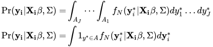
Where 
![A_{j}={\begin{cases}(-\infty ,0]&y_{j}=0\\(0,\infty )&y_{j}=1\end{cases}}](https://wikimedia.org/api/rest_v1/media/math/render/svg/3a38b27c96032c1abf5d7b979d922b8144830765)
The log-likelihood function in this case would be
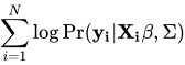
Except for 
The Multivariate Probit Model has been applied to simultaneously analyze consumer choice of multiple brands. It has been demonstrated that the Multivariate Probit model extends research possibilities in the demand area by relaxing the restrictive assumption of mutually exclusive alternatives, which characterizes multinomial discrete choice methods.
Sources and credits
This article is adapted from the Wikipedia article “Multivariate probit model”, written by its contributors and licensed under CC BY-SA 4.0. Fathomly has changed the layout, removed citation markers, navigation and maintenance notices, and adjusted punctuation. This adapted version is shared under the same license. For references, see the original article.
Fathomly is not affiliated with or endorsed by the Wikimedia Foundation. Spotted a problem? Tell us.