Encyclopedia

Multiple linear regression

Wikipedia contributorsAdapted for Fathomly · View authors

4 min read
Source updated September 14, 2026

Image credit is listed at the end of this article.

Multiple linear regression, also known as multivariable linear regression, is a generalization of simple linear regression to the case of more than one independent variable. The basic model for multiple linear regression is

$Y_{i}=\beta _{0}+\beta _{1}X_{i1}+\beta _{2}X_{i2}+\ldots +\beta _{p}X_{ip}+\epsilon _{i}$

for each observation ${\textstyle i=1,\ldots ,n$ .

In the formula above we consider n observations of one dependent variable and p independent variables. Thus, Y_i is the i^th observation of the dependent variable, X_ij is i^th observation of the j^th independent variable, j = 1, 2, ..., p. The values β_j represent parameters to be estimated, and ε_i is the i^th independent identically distributed normal error.

Nearly all real-world regression models involve multiple predictors, and basic descriptions of linear regression are often phrased in terms of the multiple regression model. Note, however, that in these cases the response variable y is still a scalar.

Multiple linear regression is a special case, restricted to one dependent variable, of general linear models (also known as multivariate linear regression), which predicts multiple correlated dependent variables.

01Formulation

Given a data set $\{y_{i},\,x_{i1},\ldots ,x_{ip}\}_{i=1}^{n}$ of n statistical units, a linear regression model assumes that the relationship between the dependent variable $y$ and the vector of regressors ${\textbf {x}}$ is linear. This relationship is modeled through a disturbance term or error variable $\varepsilon$ , an unobserved random variable that adds extra "noise" to the linear relationship between the dependent variable and regressors. Thus the model takes the form $y_{i}=\beta _{0}+\beta _{1}x_{i1}+\cdots +\beta _{p}x_{ip}+\varepsilon _{i}=\mathbf {x} _{i}^{\mathsf {T}}{\boldsymbol {\beta }}+\varepsilon _{i},\qquad i=1,\ldots ,n,$ where $^{\mathsf {T}}$ denotes the transpose, so that $\mathbf {x} _{i}^{\mathsf {T}}{\boldsymbol {\beta }}$ is the inner product between vectors $\mathbf {x} _{i}$ and ${\boldsymbol {\beta }}$ .

Often these n equations are stacked together and written in matrix notation as

$\mathbf {y} =\mathbf {X} {\boldsymbol {\beta }}+{\boldsymbol {\varepsilon }},\,$

where

$\mathbf {y} ={\begin{bmatrix}y_{1}\\y_{2}\\\vdots \\y_{n}\end{bmatrix}},\quad$

$\mathbf {X} ={\begin{bmatrix}\mathbf {x} _{1}^{\mathsf {T}}\\\mathbf {x} _{2}^{\mathsf {T}}\\\vdots \\\mathbf {x} _{n}^{\mathsf {T}}\end{bmatrix}}={\begin{bmatrix}1&x_{11}&\cdots &x_{1p}\\1&x_{21}&\cdots &x_{2p}\\\vdots &\vdots &\ddots &\vdots \\1&x_{n1}&\cdots &x_{np}\end{bmatrix}},$

${\boldsymbol {\beta }}={\begin{bmatrix}\beta _{0}\\\beta _{1}\\\beta _{2}\\\vdots \\\beta _{p}\end{bmatrix}},\quad {\boldsymbol {\varepsilon }}={\begin{bmatrix}\varepsilon _{1}\\\varepsilon _{2}\\\vdots \\\varepsilon _{n}\end{bmatrix}}.$

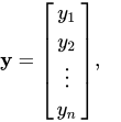
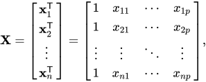
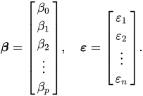
Notation and terminology

$\mathbf {y}$ is a vector of observed values $y_{i}\ (i=1,\ldots ,n)$ of the variable called the regressand, endogenous variable, response variable, target variable, measured variable, criterion variable, or dependent variable. This variable is also sometimes known as the predicted variable, but this should not be confused with predicted values, which are denoted ${\hat {y}}$ . The decision as to which variable in a data set is modeled as the dependent variable and which are modeled as the independent variables may be based on a presumption that the value of one of the variables is caused by, or directly influenced by the other variables. Alternatively, there may be an operational reason to model one of the variables in terms of the others, in which case there need be no presumption of causality.
may be seen as a matrix of row-vectors or of n-dimensional column-vectors , which are known as regressors, exogenous variables, explanatory variables, covariates, input variables, predictor variables, or independent variables (not to be confused with the concept of independent random variables). The matrix is sometimes called the design matrix.
- Usually a constant is included as one of the regressors. In particular, $x_{i0}=1$ for $i=1,\ldots ,n$ . The corresponding element of β is called the intercept. Many statistical inference procedures for linear models require an intercept to be present, so it is often included even if theoretical considerations suggest that its value should be zero.
- Sometimes one of the regressors can be a non-linear function of another regressor or of the data values, as in polynomial regression and segmented regression. The model remains linear as long as it is linear in the parameter vector β.
- The values x_ij may be viewed as either observed values of random variables X_j or as fixed values chosen prior to observing the dependent variable. Both interpretations may be appropriate in different cases, and they generally lead to the same estimation procedures; however different approaches to asymptotic analysis are used in these two situations.
${\boldsymbol {\beta }}$ is a $(p+1)$ -dimensional parameter vector, where $\beta _{0}$ is the intercept term (if one is included in the model, otherwise ${\boldsymbol {\beta }}$ is p-dimensional). Its elements are known as effects or regression coefficients (although the latter term is sometimes reserved for the estimated effects). In simple linear regression, p=1, and the coefficient is known as regression slope. Statistical estimation and inference in linear regression focuses on β. The elements of this parameter vector are interpreted as the partial derivatives of the dependent variable with respect to the various independent variables.
${\boldsymbol {\varepsilon }}$ is a vector of values $\varepsilon _{i}$ . This part of the model is called the error term, disturbance term, or sometimes noise (in contrast with the "signal" provided by the rest of the model). This variable captures all other factors which influence the dependent variable y other than the regressors x. The relationship between the error term and the regressors, for example their correlation, is a crucial consideration in formulating a linear regression model, as it will determine the appropriate estimation method.

02Solution

Fitting a linear model to a given data set usually requires estimating the regression coefficients ${\boldsymbol {\beta }}$ such that the error term ${\boldsymbol {\varepsilon }}=\mathbf {y} -\mathbf {X} {\boldsymbol {\beta }}$ is minimized. For example, it is common to use the sum of squared errors $\|{\boldsymbol {\varepsilon }}\|_{2}^{2}$ as a measure of ${\boldsymbol {\varepsilon }}$ for minimization.

03Example

Consider a situation where a small ball is being tossed up in the air and then we measure its heights of ascent h_i at various moments in time t_i. Physics tells us that, ignoring the drag, the relationship can be modeled as

$h_{i}=\beta _{1}t_{i}+\beta _{2}t_{i}^{2}+\varepsilon _{i},$

where β₁ determines the initial velocity of the ball, β₂ is proportional to the standard gravity, and ε_i is due to measurement errors. Linear regression can be used to estimate the values of β₁ and β₂ from the measured data. This model is non-linear in the time variable, but it is linear in the parameters β₁ and β₂; if we take regressors x_i = (x_i1, x_i2) = (t_i, t_i²), the model takes on the standard form

$h_{i}=\mathbf {x} _{i}^{\mathsf {T}}{\boldsymbol {\beta }}+\varepsilon _{i}.$

Watch videos about Multiple linear regressionExplainers and documentaries on YouTube (opens in a new tab)

Sources and credits

This article is adapted from the Wikipedia article “Multiple linear regression”, written by its contributors and licensed under CC BY-SA 4.0. Fathomly has changed the layout, removed citation markers, navigation and maintenance notices, and adjusted punctuation. This adapted version is shared under the same license. For references, see the original article.

Images, from Wikimedia Commons:

Linear least squares2.png by Oleg Alexandrov, Public domain

Fathomly is not affiliated with or endorsed by the Wikimedia Foundation. Spotted a problem? Tell us.

Multiple linear regression

01Formulation

Notation and terminology

02Solution

03Example

Sources and credits

Related topics

Design matrix

Linear regression

Regression analysis