Encyclopedia

Multidimensional system

System in which not only one independent variable exists

Wikipedia contributorsAdapted for Fathomly · View authors

3 min read
Source updated September 8, 2025

In mathematical systems theory, a multidimensional system or m-D system is a system in which not only one independent variable exists (like time), but there are several independent variables.

Important problems such as factorization and stability of m-D systems (m > 1) have recently attracted the interest of many researchers and practitioners. The reason is that the factorization and stability is not a straightforward extension of the factorization and stability of 1-D systems because, for example, the fundamental theorem of algebra does not exist in the ring of m-D (m > 1) polynomials.

01Applications

Multidimensional systems or m-D systems are the necessary mathematical background for modern digital image processing with many applications in biomedicine, X-ray technology and satellite communications. There are also some studies combining m-D systems with partial differential equations (PDEs).

02Linear multidimensional state-space model

A state-space model is a representation of a system in which the effect of all "prior" input values is contained by a state vector. In the case of an m-d system, each dimension has a state vector that contains the effect of prior inputs relative to that dimension. The collection of all such dimensional state vectors at a point constitutes the total state vector at the point.

Consider a uniform discrete space linear two-dimensional (2d) system that is space invariant and causal. It can be represented in matrix-vector form as follows:

Represent the input vector at each point $(i,j)$ by $u(i,j)$ , the output vector by $y(i,j)$ the horizontal state vector by $R(i,j)$ and the vertical state vector by $S(i,j)$ . Then the operation at each point is defined by:

${\begin{aligned}R(i+1,j)&=A_{1}R(i,j)+A_{2}S(i,j)+B_{1}u(i,j)\\S(i,j+1)&=A_{3}R(i,j)+A_{4}S(i,j)+B_{2}u(i,j)\\y(i,j)&=C_{1}R(i,j)+C_{2}S(i,j)+Du(i,j)\end{aligned}}$

where $A_{1},A_{2},A_{3},A_{4},B_{1},B_{2},C_{1},C_{2}$ and $D$ are matrices of appropriate dimensions.

These equations can be written more compactly by combining the matrices:

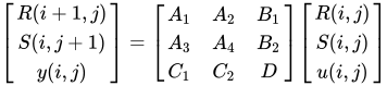
${\begin{bmatrix}R(i+1,j)\\S(i,j+1)\\y(i,j)\end{bmatrix}}={\begin{bmatrix}A_{1}&A_{2}&B_{1}\\A_{3}&A_{4}&B_{2}\\C_{1}&C_{2}&D\end{bmatrix}}{\begin{bmatrix}R(i,j)\\S(i,j)\\u(i,j)\end{bmatrix}}$

Given input vectors $u(i,j)$ at each point and initial state values, the value of each output vector can be computed by recursively performing the operation above.

03Multidimensional transfer function

A discrete linear two-dimensional system is often described by a partial difference equation in the form: $\sum _{p,q=0,0}^{m,n}a_{p,q}y(i-p,j-q)=\sum _{p,q=0,0}^{m,n}b_{p,q}x(i-p,j-q)$

where $x(i,j)$ is the input and $y(i,j)$ is the output at point $(i,j)$ and $a_{p,q}$ and $b_{p,q}$ are constant coefficients.

To derive a transfer function for the system the 2d Z-transform is applied to both sides of the equation above.

$\sum _{p,q=0,0}^{m,n}a_{p,q}z_{1}^{-p}z_{2}^{-q}Y(z_{1},z_{2})=\sum _{p,q=0,0}^{m,n}b_{p,q}z_{1}^{-p}z_{2}^{-q}X(z_{1},z_{2})$

Transposing yields the transfer function $T(z_{1},z_{2})$ :

$T(z_{1},z_{2})={Y(z_{1},z_{2}) \over X(z_{1},z_{2})}={\sum _{p,q=0,0}^{m,n}b_{p,q}z_{1}^{-p}z_{2}^{-q} \over \sum _{p,q=0,0}^{m,n}a_{p,q}z_{1}^{-p}z_{2}^{-q}}$

So given any pattern of input values, the 2d Z-transform of the pattern is computed and then multiplied by the transfer function $T(z_{1},z_{2})$ to produce the Z-transform of the system output.

04Realization of a 2d transfer function

Often an image processing or other md computational task is described by a transfer function that has certain filtering properties, but it is desired to convert it to state-space form for more direct computation. Such conversion is referred to as realization of the transfer function.

Consider a 2d linear spatially invariant causal system having an input-output relationship described by:

$Y(z_{1},z_{2})={\sum _{p,q=0,0}^{m,n}b_{p,q}z_{1}^{-p}z_{2}^{-q} \over \sum _{p,q=0,0}^{m,n}a_{p,q}z_{1}^{-p}z_{2}^{-q}}X(z_{1},z_{2})$

Two cases are individually considered 1) the bottom summation is simply the constant 1 2) the top summation is simply a constant $k$ . Case 1 is often called the "all-zero" or "finite impulse response" case, whereas case 2 is called the "all-pole" or "infinite impulse response" case. The general situation can be implemented as a cascade of the two individual cases. The solution for case 1 is considerably simpler than case 2 and is shown below.

Example: all zero or finite impulse response

$Y(z_{1},z_{2})=\sum _{p,q=0,0}^{m,n}b_{p,q}z_{1}^{-p}z_{2}^{-q}X(z_{1},z_{2})$

The state-space vectors will have the following dimensions:

$R(1\times m),\quad S(1\times n),\quad x(1\times 1)$ and $y(1\times 1)$

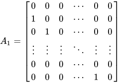
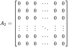
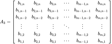
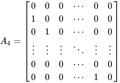
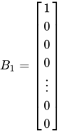
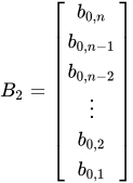
Each term in the summation involves a negative (or zero) power of $z_{1}$ and of $z_{2}$ which correspond to a delay (or shift) along the respective dimension of the input $x(i,j)$ . This delay can be effected by placing $1$ ’s along the super diagonal in the $A_{1}$ . and $A_{4}$ matrices and the multiplying coefficients $b_{i,j}$ in the proper positions in the $A_{2}$ . The value $b_{0,0}$ is placed in the upper position of the $B_{1}$ matrix, which will multiply the input $x(i,j)$ and add it to the first component of the $R_{i,j}$ vector. Also, a value of $b_{0,0}$ is placed in the $D$ matrix which will multiply the input $x(i,j)$ and add it to the output $y$ . The matrices then appear as follows:

$A_{1}={\begin{bmatrix}0&0&0&\cdots &0&0\\1&0&0&\cdots &0&0\\0&1&0&\cdots &0&0\\\vdots &\vdots &\vdots &\ddots &\vdots &\vdots \\0&0&0&\cdots &0&0\\0&0&0&\cdots &1&0\end{bmatrix}}$

$A_{2}={\begin{bmatrix}0&0&0&\cdots &0&0\\0&0&0&\cdots &0&0\\0&0&0&\cdots &0&0\\\vdots &\vdots &\vdots &\ddots &\vdots &\vdots \\0&0&0&\cdots &0&0\\0&0&0&\cdots &0&0\end{bmatrix}}$

$A_{3}={\begin{bmatrix}b_{1,n}&b_{2,n}&b_{3,n}&\cdots &b_{m-1,n}&b_{m,n}\\b_{1,n-1}&b_{2,n-1}&b_{3,n-1}&\cdots &b_{m-1,n-1}&b_{m,n-1}\\b_{1,n-2}&b_{2,n-2}&b_{3,n-2}&\cdots &b_{m-1,n-2}&b_{m,n-2}\\\vdots &\vdots &\vdots &\ddots &\vdots &\vdots \\b_{1,2}&b_{2,2}&b_{3,2}&\cdots &b_{m-1,2}&b_{m,2}\\b_{1,1}&b_{2,1}&b_{3,1}&\cdots &b_{m-1,1}&b_{m,1}\end{bmatrix}}$

$A_{4}={\begin{bmatrix}0&0&0&\cdots &0&0\\1&0&0&\cdots &0&0\\0&1&0&\cdots &0&0\\\vdots &\vdots &\vdots &\ddots &\vdots &\vdots \\0&0&0&\cdots &0&0\\0&0&0&\cdots &1&0\end{bmatrix}}$

$B_{1}={\begin{bmatrix}1\\0\\0\\0\\\vdots \\0\\0\end{bmatrix}}$

$B_{2}={\begin{bmatrix}b_{0,n}\\b_{0,n-1}\\b_{0,n-2}\\\vdots \\b_{0,2}\\b_{0,1}\end{bmatrix}}$

$C_{1}={\begin{bmatrix}b_{1,0}&b_{2,0}&b_{3,0}&\cdots &b_{m-1,0}&b_{m,0}\\\end{bmatrix}}$

$C_{2}={\begin{bmatrix}0&0&0&\cdots &0&1\\\end{bmatrix}}$

$D={\begin{bmatrix}b_{0,0}\end{bmatrix}}$

Watch videos about Multidimensional systemExplainers and documentaries on YouTube (opens in a new tab)

Sources and credits

This article is adapted from the Wikipedia article “Multidimensional system”, written by its contributors and licensed under CC BY-SA 4.0. Fathomly has changed the layout, removed citation markers, navigation and maintenance notices, and adjusted punctuation. This adapted version is shared under the same license. For references, see the original article.

Fathomly is not affiliated with or endorsed by the Wikimedia Foundation. Spotted a problem? Tell us.