Encyclopedia

Moving load

Load that changes in time

Wikipedia contributorsAdapted for Fathomly · View authors

2 min read
Source updated October 3, 2025

Image credit is listed at the end of this article.

In structural dynamics, a moving load changes the point at which the load is applied over time. Examples include a vehicle that travels across a bridge and a train moving along a track.

01Properties

In computational models, load is usually applied as

a simple massless force,
an oscillator, or
an inertial force (mass and a massless force).

Numerous historical reviews of the moving load problem exist. Several publications deal with similar problems.

The fundamental monograph is devoted to massless loads. Inertial load in numerical models is described in

Unexpected property of differential equations that govern the motion of the mass particle travelling on the string, Timoshenko beam, and Mindlin plate is described in. It is the discontinuity of the mass trajectory near the end of the span (well visible in string at the speed v=0.5c). The moving load significantly increases displacements. The critical velocity, at which the growth of displacements is the maximum, must be taken into account in engineering projects.

Structures that carry moving loads can have finite dimensions or can be infinite and supported periodically or placed on the elastic foundation.

Consider simply supported string of the length l, cross-sectional area A, mass density ρ, tensile force N, subjected to a constant force P moving with constant velocity v. The motion equation of the string under the moving force has a form

$-N{\frac {\partial ^{2}w(x,t)}{\partial x^{2}}}+\rho A{\frac {\partial ^{2}w(x,t)}{\partial t^{2}}}=\delta (x-vt)P\ .$

Displacements of any point of the simply supported string is given by the sinus series

$w(x,t)={\frac {2P}{\rho Al}}\sum _{j=1}^{\infty }{\frac {1}{\omega _{(j)}^{2}-\omega ^{2}}}\left(\sin(\omega t)-{\frac {\omega }{\omega _{(j)}}}\sin(\omega _{(j)}t)\right)\sin {\frac {j\pi x}{l}}\ ,$

where

$\omega ={\frac {j\pi v}{l}}\ ,$

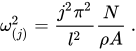
and the natural circular frequency of the string

$\omega _{(j)}^{2}={\frac {j^{2}\pi ^{2}}{l^{2}}}{\frac {N}{\rho A}}\ .$

In the case of inertial moving load, the analytical solutions are unknown. The equation of motion is increased by the term related to the inertia of the moving load. A concentrated mass m accompanied by a point force P:

$-N{\frac {\partial ^{2}w(x,t)}{\partial x^{2}}}+\rho A{\frac {\partial ^{2}w(x,t)}{\partial t^{2}}}=\delta (x-vt)P-\delta (x-vt)m{\frac {{\mbox{d}}^{2}w(vt,t)}{{\mbox{d}}t^{2}}}\ .$

The last term, because of complexity of computations, is often neglected by engineers. The load influence is reduced to the massless load term. Sometimes the oscillator is placed in the contact point. Such approaches are acceptable only in low range of the travelling load velocity. In higher ranges both the amplitude and the frequency of vibrations differ significantly in the case of both types of a load.

The differential equation can be solved in a semi-analytical way only for simple problems. The series determining the solution converges well and 2-3 terms are sufficient in practice. More complex problems can be solved by the finite element method or space-time finite element method.

massless load	inertial load

The discontinuity of the mass trajectory is also well visible in the Timoshenko beam. High shear stiffness emphasizes the phenomenon.

Vibrations of a string under a moving massless force (v=0.1c); c is the wave speed.

Vibrations of a string under a moving massless force (v=0.5c); c is the wave speed.

Vibrations of a string under a moving inertial force (v=0.1c); c is the wave speed.

02Massless string under moving inertial load

Consider a massless string, which is a particular case of moving inertial load problem. The first to solve the problem was Smith. The analysis will follow the solution of Fryba. Assuming ρ=0, the equation of motion of a string under a moving mass can be put into the following form

$-N{\frac {\partial ^{2}w(x,t)}{\partial x^{2}}}=\delta (x-vt)P-\delta (x-vt)\,m{\frac {{\mbox{d}}^{2}w(vt,t)}{{\mbox{d}}t^{2}}}\ .$

We impose simply-supported boundary conditions and zero initial conditions. To solve this equation we use the convolution property. We assume dimensionless displacements of the string y and dimensionless time τ:

$y(\tau )={\frac {w(vt,t)}{w_{st}}}\ ,\ \ \ \ \tau \ =\ {\frac {vt}{l}}\ ,$

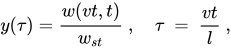
where w_st is the static deflection in the middle of the string. The solution is given by a sum

$y(\tau )={\frac {4\,\alpha }{\alpha \,-\,1}}\,\tau \,(\tau -1)\,\sum _{k=1}^{\infty }\,\prod _{i=1}^{k}{\frac {(a+i-1)(b+i-1)}{c+i-1}}\;{\frac {\tau ^{k}}{k!}}\ ,$

where α is the dimensionless parameters :

$\alpha ={\frac {Nl}{2mv2}}\,>\,0\ \ \ \wedge \ \ \ \alpha \,\neq \,1\ .$

Parameters a, b and c are given below

$a_{1,2}={\frac {3\,\pm \,{\sqrt {1+8\alpha }}}{2}}\ ,\ \ \ \ \ b_{1,2}={\frac {3\,\mp \,{\sqrt {1+8\alpha }}}{2}}\ ,\ \ \ \ \ c=2\ .$

In the case of α=1, the considered problem has a closed solution: $y(\tau )=\left[{\frac {4}{3}}\tau (1-\tau )-{\frac {4}{3}}\tau \left(1+2\tau \ln(1-\tau )+2\ln(1-\tau )\right)\right]\ .$

Vibrations of a string under a moving inertial force (v=0.5c); c is the wave speed.

Vibrations of the Timoshenko beam: red lines - beam axes in time, black line - mass trajectory (w0- static deflection).

Watch videos about Moving loadExplainers and documentaries on YouTube (opens in a new tab)

Sources and credits

This article is adapted from the Wikipedia article “Moving load”, written by its contributors and licensed under CC BY-SA 4.0. Fathomly has changed the layout, removed citation markers, navigation and maintenance notices, and adjusted punctuation. This adapted version is shared under the same license. For references, see the original article.

Images, from Wikimedia Commons:

Cb pant.png by Cbajer, CC BY-SA 3.0
Stru mody kol.png by Cbajer, CC BY-SA 3.0
Wiki01f50.gif by Cbajer, CC BY-SA 3.0
Wiki05f50.gif by Cbajer, CC BY-SA 3.0
Wiki01m50.gif by Cbajer, CC BY-SA 3.0
Wiki05m50.gif by Cbajer, CC BY-SA 3.0
Timo04n.png by Cbajer, CC BY-SA 3.0
Wiki rozero kol.png by Cbajer, CC BY-SA 3.0
Wiki alfa1 kol.png by Cbajer, CC BY-SA 3.0

Fathomly is not affiliated with or endorsed by the Wikimedia Foundation. Spotted a problem? Tell us.