Metabolic control analysis
Mathematical model of biochemical pathways

In biochemistry, metabolic control analysis (MCA) is a mathematical framework for describing metabolic, signaling, and genetic pathways. MCA quantifies how variables, such as fluxes and species concentrations, depend on network parameters. In particular, it is able to describe how network-dependent properties, called control coefficients, depend on local properties called elasticities or elasticity coefficients.
MCA was originally developed to describe the control in metabolic pathways but was subsequently extended to describe signaling and genetic networks. MCA has sometimes also been referred to as Metabolic Control Theory, but this terminology was rather strongly opposed by Henrik Kacser, one of the founders.
More recent work has shown that MCA can be mapped directly on to classical control theory and are as such equivalent.
Biochemical systems theory (BST) is a similar formalism, though with rather different objectives. Both are evolutions of an earlier theoretical analysis by Joseph Higgins.
Chemical reaction network theory is another theoretical framework that has overlap with both MCA and BST but is considerably more mathematically formal in its approach. Its emphasis is primarily on dynamic stability criteria and related theorems associated with mass-action networks. In more recent years the field has also developed a sensitivity analysis which is similar if not identical to MCA and BST.
01Control coefficients
A control coefficient
measures the relative steady state change in a system variable, e.g. pathway flux (J) or metabolite concentration (S), in response to a relative change in a parameter, e.g. enzyme activity or the steady-state rate (


and concentration control coefficients by

.
Summation theorems
The flux control summation theorem was discovered independently by the Kacser/Burns group and the Heinrich/Rapoport group in the early 1970s and late 1960s. The flux control summation theorem implies that metabolic fluxes are systemic properties and that their control is shared by all reactions in the system. When a single reaction changes its control of the flux this is compensated by changes in the control of the same flux by all other reactions.


Elasticity coefficients
The elasticity coefficient measures the local response of an enzyme or other chemical reaction to changes in its environment. Such changes include factors such as substrates, products, or effector concentrations. For further information, please refer to the dedicated page at elasticity coefficients.
.
Connectivity theorems
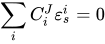
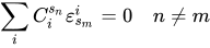
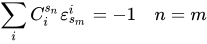
The connectivity theorems are specific relationships between elasticities and control coefficients. They are useful because they highlight the close relationship between the kinetic properties of individual reactions and the system properties of a pathway. Two basic sets of theorems exists, one for flux and another for concentrations. The concentration connectivity theorems are divided again depending on whether the system species 


02Response Coefficient
Kacser and Burns introduced an additional coefficient that described how a biochemical pathway would respond the external environment. They termed this coefficient the response coefficient and designated it using the symbol R. The response coefficient is an important metric because it can be used to assess how much a nutrient or perhaps more important, how a drug can influence a pathway. This coefficient is therefore highly relevant to the pharmaceutical industry.
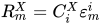
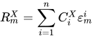
The response coefficient is related to the core of metabolic control analysis via the response coefficient theorem, which is stated as follows:
where 


The key observation of this theorem is that an external factor such as a therapeutic drug, acts on the organism's phenotype via two influences: 1) How well the drug can affect the target itself through effective binding of the drug to the target protein and its effect on the protein activity. This effectiveness is described by the elasticity
A drug action, or any external factor, is most effective when both these factors are strong. For example, a drug might be very effective at changing the activity of its target protein, however if that perturbation in protein activity is unable to be transmitted to the final phenotype then the effectiveness of the drug is greatly diminished.
If a drug or external factor, 
03Control equations
It is possible to combine the summation with the connectivity theorems to obtain closed expressions that relate the control coefficients to the elasticity coefficients. For example, consider the simplest non-trivial pathway:

We assume that 


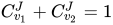

Using these two equations we can solve for the flux control coefficients to yield
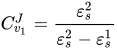
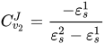
Using these equations we can look at some simple extreme behaviors. For example, let us assume that the first step is completely insensitive to its product (i.e. not reacting with it), S, then 


That is all the control (or sensitivity) is on the first step. This situation represents the classic rate-limiting step that is frequently mentioned in textbooks. The flux through the pathway is completely dependent on the first step. Under these conditions, no other step in the pathway can affect the flux. The effect is however dependent on the complete insensitivity of the first step to its product. Such a situation is likely to be rare in real pathways. In fact the classic rate limiting step has almost never been observed experimentally. Instead, a range of limitingness is observed, with some steps having more limitingness (control) than others.
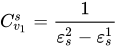
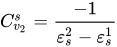
We can also derive the concentration control coefficients for the simple two step pathway:
04Three step pathway
Consider the simple three step pathway:

where
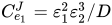

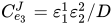
where D the denominator is given by

Note that every term in the numerator appears in the denominator, this ensures that the flux control coefficient summation theorem is satisfied.
Likewise the concentration control coefficients can also be derived, for

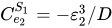

And for

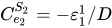

Note that the denominators remain the same as before and behave as a normalizing factor.

05Derivation using perturbations
Control equations can also be derived by considering the effect of perturbations on the system. Consider that reaction rates 


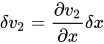
where the derivative 


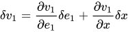
We have two equations, one describing the change in 
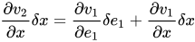
Solving for the ratio 
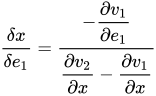
In the limit, as we make the change 
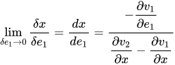
We can go one step further and scale the derivatives to eliminate units. Multiplying both sides by
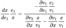
The scaled derivatives on the right-hand side are the elasticities, 

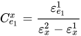
We can simplify this expression further. The reaction rate 

Using this result gives:
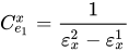
A similar analysis can be done where
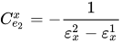
The above expressions measure how much enzymes 



The above expressions tell us how much enzymes
06Derivation using the systems equation
The control equations can also be derived in a more rigorous fashion using the systems equation:
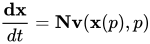
where 


07Properties of a linear pathway
A linear biochemical pathway is a chain of enzyme-catalyzed reaction steps. The figure below shows a three step pathway, with intermediates, 

At steady-state the rate of reaction is the same at each step. This means there is an overall flux from X_o to X_1.
Linear pathways possess some well-known properties:
- Flux control is biased towards the first few steps of the pathway. Flux control shifts more to the first step as the equilibrium constants become large.
- Flux control is small at reactions close to equilibrium.
- Assuming reversibly, flux control at a given step is proportional to the product of the equilibrium constants. For example, flux control at the second step in a three step pathway is proportional to the product of the second and third equilibrium constants.
In all cases, a rationale for these behaviors is given in terms of how elasticities transmit changes through a pathway.

08Metabolic control analysis software
There are a number of software tools that can directly compute elasticities and control coefficients:
- COPASI (GUI)
- PySCeS (Python)
- SBW (GUI)
- libroadrunner (Python)
- VCell
09Relationship to Classical Control Theory
Classical Control theory is a field of mathematics that deals with the control of dynamical systems in engineered processes and machines. In 2004 Brian Ingalls published a paper that showed that classical control theory and metabolic control analysis were identical. The only difference was that metabolic control analysis was confined to zero frequency responses when cast in the frequency domain whereas classical control theory imposes no such restriction. The other significant difference is that classical control theory has no notion of stoichiometry and conservation of mass which makes it more cumbersome to use but also means it fails to recognize the structural properties inherent in stoichiometric networks which provide useful biological insights.
Sources and credits
This article is adapted from the Wikipedia article “Metabolic control analysis”, written by its contributors and licensed under CC BY-SA 4.0. Fathomly has changed the layout, removed citation markers, navigation and maintenance notices, and adjusted punctuation. This adapted version is shared under the same license. For references, see the original article.
Images, from Wikimedia Commons:
- MCAlogo.png by Rhodydog, CC BY-SA 4.0
- SystemControl.png by Rhodydog, CC BY-SA 4.0
- LocalControl.png by Rhodydog, CC BY-SA 4.0
- Linear3Step.png by rhodydog, CC0
Fathomly is not affiliated with or endorsed by the Wikimedia Foundation. Spotted a problem? Tell us.
