Encyclopedia

Manifold regularization

Technique for shaping training datasets

Wikipedia contributorsAdapted for Fathomly · View authors

7 min read
Source updated November 30, 2025

Image credit is listed at the end of this article.

In machine learning, manifold regularization is a technique for using the shape of a dataset to constrain the functions that should be learned on that dataset. In many machine learning problems, the data to be learned do not cover the entire input space. For example, a facial recognition system may not need to classify any possible image, but only the subset of images that contain faces. The technique of manifold learning assumes that the relevant subset of data comes from a manifold, a mathematical structure with useful properties. The technique also assumes that the function to be learned is smooth: data with different labels are not likely to be close together, and so the labeling function should not change quickly in areas where there are likely to be many data points. Because of this assumption, a manifold regularization algorithm can use unlabeled data to inform where the learned function is allowed to change quickly and where it is not, using an extension of the technique of Tikhonov regularization. Manifold regularization algorithms can extend supervised learning algorithms in semi-supervised learning and transductive learning settings, where unlabeled data are available. The technique has been used for applications including medical imaging, geographical imaging, and object recognition.

01Manifold regularizer

Motivation

Manifold regularization is a type of regularization, a family of techniques that reduces overfitting and ensures that a problem is well-posed by penalizing complex solutions. In particular, manifold regularization extends the technique of Tikhonov regularization as applied to Reproducing kernel Hilbert spaces (RKHSs). Under standard Tikhonov regularization on RKHSs, a learning algorithm attempts to learn a function $f$ from among a hypothesis space of functions ${\mathcal {H}}$ . The hypothesis space is an RKHS, meaning that it is associated with a kernel $K$ , and so every candidate function $f$ has a norm $\left\|f\right\|_{K}$ , which represents the complexity of the candidate function in the hypothesis space. When the algorithm considers a candidate function, it takes its norm into account in order to penalize complex functions.

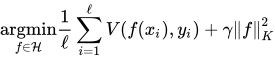
Formally, given a set of labeled training data $(x_{1},y_{1}),\ldots ,(x_{\ell },y_{\ell })$ with $x_{i}\in X,y_{i}\in Y$ and a loss function $V$ , a learning algorithm using Tikhonov regularization will attempt to solve the expression

${\underset {f\in {\mathcal {H}}}{\arg \!\min }}{\frac {1}{\ell }}\sum _{i=1}^{\ell }V(f(x_{i}),y_{i})+\gamma \left\|f\right\|_{K}^{2}$

where $\gamma$ is a hyperparameter that controls how much the algorithm will prefer simpler functions over functions that fit the data better.

Manifold regularization adds a second regularization term, the intrinsic regularizer, to the ambient regularizer used in standard Tikhonov regularization. Under the manifold assumption in machine learning, the data in question do not come from the entire input space $X$ , but instead from a nonlinear manifold $M\subset X$ . The geometry of this manifold, the intrinsic space, is used to determine the regularization norm.

Laplacian norm

There are many possible choices for the intrinsic regularizer $\left\|f\right\|_{I}$ . Many natural choices involve the gradient on the manifold $\nabla _{M}$ , which can provide a measure of how smooth a target function is. A smooth function should change slowly where the input data are dense; that is, the gradient $\nabla _{M}f(x)$ should be small where the marginal probability density ${\mathcal {P}}_{X}(x)$ , the probability density of a randomly drawn data point appearing at $x$ , is large. This gives one appropriate choice for the intrinsic regularizer:

$\left\|f\right\|_{I}^{2}=\int _{x\in M}\left\|\nabla _{M}f(x)\right\|^{2}\,d{\mathcal {P}}_{X}(x)$

In practice, this norm cannot be computed directly because the marginal distribution ${\mathcal {P}}_{X}$ is unknown, but it can be estimated from the provided data.

Graph-based approach of the Laplacian norm

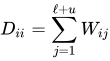
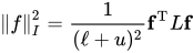
When the distances between input points are interpreted as a graph, then the Laplacian matrix of the graph can help to estimate the marginal distribution. Suppose that the input data include $\ell$ labeled examples (pairs of an input $x$ and a label $y$ ) and $u$ unlabeled examples (inputs without associated labels). Define $W$ to be a matrix of edge weights for a graph, where $W_{ij}$ is a similarity built from distance measure between the data points $x_{i}$ and $x_{j}$ (so that more close implies higher $W_{ij}$ ). Define $D$ to be a diagonal matrix with $D_{ii}=\sum _{j=1}^{\ell +u}W_{ij}$ and $L$ to be the Laplacian matrix $D-W$ . Then, as the number of data points $\ell +u$ increases, $L$ converges to the Laplace-Beltrami operator $\Delta _{M}$ , which is the divergence of the gradient $\nabla _{M}$ . Then, if $\mathbf {f}$ is a vector of the values of $f$ at the data, $\mathbf {f} =[f(x_{1}),\ldots ,f(x_{l+u})]^{\mathrm {T} }$ , the intrinsic norm can be estimated:

$\left\|f\right\|_{I}^{2}={\frac {1}{(\ell +u)^{2}}}\mathbf {f} ^{\mathrm {T} }L\mathbf {f}$

As the number of data points $\ell +u$ increases, this empirical definition of $\left\|f\right\|_{I}^{2}$ converges to the definition when ${\mathcal {P}}_{X}$ is known.

Solving the regularization problem with graph-based approach

Using the weights $\gamma _{A}$ and $\gamma _{I}$ for the ambient and intrinsic regularizers, the final expression to be solved becomes:

${\underset {f\in {\mathcal {H}}}{\arg \!\min }}{\frac {1}{\ell }}\sum _{i=1}^{\ell }V(f(x_{i}),y_{i})+\gamma _{A}\left\|f\right\|_{K}^{2}+{\frac {\gamma _{I}}{(\ell +u)^{2}}}\mathbf {f} ^{\mathrm {T} }L\mathbf {f}$

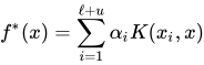
As with other kernel methods, ${\mathcal {H}}$ may be an infinite-dimensional space, so if the regularization expression cannot be solved explicitly, it is impossible to search the entire space for a solution. Instead, a representer theorem shows that under certain conditions on the choice of the norm $\left\|f\right\|_{I}$ , the optimal solution $f^{*}$ must be a linear combination of the kernel centered at each of the input points: for some weights $\alpha _{i}$ ,

$f^{*}(x)=\sum _{i=1}^{\ell +u}\alpha _{i}K(x_{i},x)$

Using this result, it is possible to search for the optimal solution $f^{*}$ by searching the finite-dimensional space defined by the possible choices of $\alpha _{i}$ .

Functional approach of the Laplacian norm

The idea beyond the graph-Laplacian is to use neighbors to estimate the Laplacian. This method is akin to local averaging methods, that are known to scale poorly in high-dimensional problems. Indeed, the graph Laplacian is known to suffer from the curse of dimensionality. Luckily, it is possible to leverage expected smoothness of the function to estimate thanks to more advanced functional analysis. This method consists of estimating the Laplacian operator using derivatives of the kernel reading $\partial _{1,j}K(x_{i},x)$ where $\partial _{1,j}$ denotes the partial derivatives according to the j-th coordinate of the first variable. This second approach to the Laplacian norm is to put in relation with meshfree methods, that contrast with the finite difference method in PDE.

02Applications

Manifold regularization can extend a variety of algorithms that can be expressed using Tikhonov regularization, by choosing an appropriate loss function $V$ and hypothesis space ${\mathcal {H}}$ . Two commonly used examples are the families of support vector machines and regularized least squares algorithms. (Regularized least squares includes the ridge regression algorithm; the related algorithms of LASSO and elastic net regularization can be expressed as support vector machines.) The extended versions of these algorithms are called Laplacian Regularized Least Squares (abbreviated LapRLS) and Laplacian Support Vector Machines (LapSVM), respectively.

Laplacian Regularized Least Squares (LapRLS)

Regularized least squares (RLS) is a family of regression algorithms: algorithms that predict a value $y=f(x)$ for its inputs $x$ , with the goal that the predicted values should be close to the true labels for the data. In particular, RLS is designed to minimize the mean squared error between the predicted values and the true labels, subject to regularization. Ridge regression is one form of RLS; in general, RLS is the same as ridge regression combined with the kernel method. The problem statement for RLS results from choosing the loss function $V$ in Tikhonov regularization to be the mean squared error:

$f^{*}={\underset {f\in {\mathcal {H}}}{\arg \!\min }}{\frac {1}{\ell }}\sum _{i=1}^{\ell }(f(x_{i})-y_{i})^{2}+\gamma \left\|f\right\|_{K}^{2}$

Thanks to the representer theorem, the solution can be written as a weighted sum of the kernel evaluated at the data points:

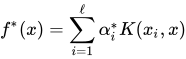
$f^{*}(x)=\sum _{i=1}^{\ell }\alpha _{i}^{*}K(x_{i},x)$

and solving for $\alpha ^{*}$ gives:

$\alpha ^{*}=(K+\gamma \ell I)^{-1}Y$

where $K$ is defined to be the kernel matrix, with $K_{ij}=K(x_{i},x_{j})$ , and $Y$ is the vector of data labels.

Adding a Laplacian term for manifold regularization gives the Laplacian RLS statement:

$f^{*}={\underset {f\in {\mathcal {H}}}{\arg \!\min }}{\frac {1}{\ell }}\sum _{i=1}^{\ell }(f(x_{i})-y_{i})^{2}+\gamma _{A}\left\|f\right\|_{K}^{2}+{\frac {\gamma _{I}}{(\ell +u)^{2}}}\mathbf {f} ^{\mathrm {T} }L\mathbf {f}$

The representer theorem for manifold regularization again gives

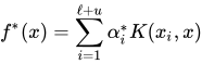
$f^{*}(x)=\sum _{i=1}^{\ell +u}\alpha _{i}^{*}K(x_{i},x)$

and this yields an expression for the vector $\alpha ^{*}$ . Letting $K$ be the kernel matrix as above, $Y$ be the vector of data labels, and $J$ be the $(\ell +u)\times (\ell +u)$ block matrix ${\begin{bmatrix}I_{\ell }&0\\0&0_{u}\end{bmatrix}}$ :

$\alpha ^{*}={\underset {\alpha \in \mathbf {R} ^{\ell +u}}{\arg \!\min }}{\frac {1}{\ell }}(Y-JK\alpha )^{\mathrm {T} }(Y-JK\alpha )+\gamma _{A}\alpha ^{\mathrm {T} }K\alpha +{\frac {\gamma _{I}}{(\ell +u)^{2}}}\alpha ^{\mathrm {T} }KLK\alpha$

with a solution of

$\alpha ^{*}=\left(JK+\gamma _{A}\ell I+{\frac {\gamma _{I}\ell }{(\ell +u)^{2}}}LK\right)^{-1}Y$

LapRLS has been applied to problems including sensor networks, medical imaging, object detection, spectroscopy, document classification, drug-protein interactions, and compressing images and videos.

Laplacian Support Vector Machines (LapSVM)

Support vector machines (SVMs) are a family of algorithms often used for classifying data into two or more groups, or classes. Intuitively, an SVM draws a boundary between classes so that the closest labeled examples to the boundary are as far away as possible. This can be directly expressed as a linear program, but it is also equivalent to Tikhonov regularization with the hinge loss function, $V(f(x),y)=\max(0,1-yf(x))$ :

$f^{*}={\underset {f\in {\mathcal {H}}}{\arg \!\min }}{\frac {1}{\ell }}\sum _{i=1}^{\ell }\max(0,1-y_{i}f(x_{i}))+\gamma \left\|f\right\|_{K}^{2}$

Adding the intrinsic regularization term to this expression gives the LapSVM problem statement:

$f^{*}={\underset {f\in {\mathcal {H}}}{\arg \!\min }}{\frac {1}{\ell }}\sum _{i=1}^{\ell }\max(0,1-y_{i}f(x_{i}))+\gamma _{A}\left\|f\right\|_{K}^{2}+{\frac {\gamma _{I}}{(\ell +u)^{2}}}\mathbf {f} ^{\mathrm {T} }L\mathbf {f}$

Again, the representer theorem allows the solution to be expressed in terms of the kernel evaluated at the data points:

$f^{*}(x)=\sum _{i=1}^{\ell +u}\alpha _{i}^{*}K(x_{i},x)$

$\alpha$ can be found by writing the problem as a linear program and solving the dual problem. Again letting $K$ be the kernel matrix and $J$ be the block matrix ${\begin{bmatrix}I_{\ell }&0\\0&0_{u}\end{bmatrix}}$ , the solution can be shown to be

$\alpha =\left(2\gamma _{A}I+2{\frac {\gamma _{I}}{(\ell +u)^{2}}}LK\right)^{-1}J^{\mathrm {T} }Y\beta ^{*}$

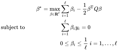
where $\beta ^{*}$ is the solution to the dual problem

${\begin{aligned}&&\beta ^{*}=\max _{\beta \in \mathbf {R} ^{\ell }}&\sum _{i=1}^{\ell }\beta _{i}-{\frac {1}{2}}\beta ^{\mathrm {T} }Q\beta \\&{\text{subject to}}&&\sum _{i=1}^{\ell }\beta _{i}y_{i}=0\\&&&0\leq \beta _{i}\leq {\frac {1}{\ell }}\;i=1,\ldots ,\ell \end{aligned}}$

and $Q$ is defined by

$Q=YJK\left(2\gamma _{A}I+2{\frac {\gamma _{I}}{(\ell +u)^{2}}}LK\right)^{-1}J^{\mathrm {T} }Y$

LapSVM has been applied to problems including geographical imaging, medical imaging, face recognition, machine maintenance, and brain-computer interfaces.

03Limitations

Manifold regularization assumes that data with different labels are not likely to be close together. This assumption is what allows the technique to draw information from unlabeled data, but it only applies to some problem domains. Depending on the structure of the data, it may be necessary to use a different semi-supervised or transductive learning algorithm.
In some datasets, the intrinsic norm of a function $\left\|f\right\|_{I}$ can be very close to the ambient norm $\left\|f\right\|_{K}$ : for example, if the data consist of two classes that lie on perpendicular lines, the intrinsic norm will be equal to the ambient norm. In this case, unlabeled data have no effect on the solution learned by manifold regularization, even if the data fit the algorithm's assumption that the separator should be smooth. Approaches related to co-training have been proposed to address this limitation.
If there are a very large number of unlabeled examples, the kernel matrix $K$ becomes very large, and a manifold regularization algorithm may become prohibitively slow to compute. Online algorithms and sparse approximations of the manifold may help in this case.

Watch videos about Manifold regularizationExplainers and documentaries on YouTube (opens in a new tab)

Sources and credits

This article is adapted from the Wikipedia article “Manifold regularization”, written by its contributors and licensed under CC BY-SA 4.0. Fathomly has changed the layout, removed citation markers, navigation and maintenance notices, and adjusted punctuation. This adapted version is shared under the same license. For references, see the original article.

Images, from Wikimedia Commons:

Example of unlabeled data in semisupervised learning.png by Techerin, CC BY-SA 3.0
Swissroll manifold unrolled.png by Olivier Grisel, CC BY 3.0

Fathomly is not affiliated with or endorsed by the Wikimedia Foundation. Spotted a problem? Tell us.