Encyclopedia

Magnetic current

Flow of magnetic monopole charge

Wikipedia contributorsAdapted for Fathomly · View authors

2 min read
Source updated March 5, 2024

Magnetic current is, nominally, a current composed of moving magnetic monopoles. It has the unit volt. The usual symbol for magnetic current is $k$ , which is analogous to $i$ for electric current. Magnetic currents produce an electric field analogously to the production of a magnetic field by electric currents. Magnetic current density, which has the unit V/m² (volt per square meter), is usually represented by the symbols ${\mathfrak {M}}^{\text{t}}$ and ${\mathfrak {M}}^{\text{i}}$ . The superscripts indicate total and impressed magnetic current density. The impressed currents are the energy sources. In many useful cases, a distribution of electric charge can be mathematically replaced by an equivalent distribution of magnetic current. This artifice can be used to simplify some electromagnetic field problems. It is possible to use both electric current densities and magnetic current densities in the same analysis.

The direction of the electric field produced by magnetic currents is determined by the left-hand rule (opposite direction as determined by the right-hand rule) as evidenced by the negative sign in the equation $\nabla \times {\mathcal {E}}=-{\mathfrak {M}}^{\text{t}}.$

01Magnetic displacement current

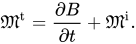
Magnetic displacement current or more properly the magnetic displacement current density is the familiar term ∂B/∂t It is one component of ${\mathfrak {M}}^{\text{t}}$ . ${\mathfrak {M}}^{\text{t}}={\frac {\partial B}{\partial t}}+{\mathfrak {M}}^{\text{i}}.$ where

${\mathfrak {M}}^{\text{t}}$ is the total magnetic current.
${\mathfrak {M}}^{\text{i}}$ is the impressed magnetic current (energy source).

02Electric vector potential

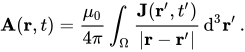
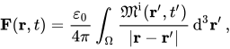
The electric vector potential, F, is computed from the magnetic current density, ${\mathfrak {M}}^{\text{i}}$ , in the same way that the magnetic vector potential, A, is computed from the electric current density. Examples of use include finite diameter wire antennas and transformers.

magnetic vector potential: $\mathbf {A} (\mathbf {r} ,t)={\frac {\mu _{0}}{4\pi }}\int _{\Omega }{\frac {\mathbf {J} (\mathbf {r} ',t')}{|\mathbf {r} -\mathbf {r} '|}}\,\mathrm {d} ^{3}\mathbf {r} '\,.$

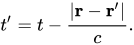
electric vector potential: $\mathbf {F} (\mathbf {r} ,t)={\frac {\varepsilon _{0}}{4\pi }}\int _{\Omega }{\frac {{\mathfrak {M}}^{\text{i}}(\mathbf {r} ',t')}{|\mathbf {r} -\mathbf {r} '|}}\,\mathrm {d} ^{3}\mathbf {r} '\,,$ where F at point $\mathbf {r}$ and time $t$ is calculated from magnetic currents at distant position $\mathbf {r} '$ at an earlier time $t'$ . The location $\mathbf {r} '$ is a source point within volume Ω that contains the magnetic current distribution. The integration variable, $\mathrm {d} ^{3}\mathbf {r} '$ , is a volume element around position $\mathbf {r} '$ . The earlier time $t'$ is called the retarded time, and calculated as $t'=t-{\frac {|\mathbf {r} -\mathbf {r} '|}{c}}.$

Retarded time accounts for the accounts for the time required for electromagnetic effects to propagate from point $\mathbf {r} '$ to point $\mathbf {r}$ .

Phasor form

When all the functions of time are sinusoids of the same frequency, the time domain equation can be replaced with a frequency domain equation. Retarded time is replaced with a phase term. $\mathbf {F} (\mathbf {r} )={\frac {\varepsilon _{0}}{4\pi }}\int _{\Omega }{\frac {{\mathfrak {M}}^{\text{i}}(\mathbf {r} )e^{-jk|\mathbf {r} -\mathbf {r} '|}}{|\mathbf {r} -\mathbf {r} '|}}\,\mathrm {d} ^{3}\mathbf {r} '\,,$ where $\mathbf {F}$ and ${\mathfrak {M}}^{\text{i}}$ are phasor quantities and $k$ is the wave number.

03Magnetic frill generator

A distribution of magnetic current, commonly called a magnetic frill generator, may be used to replace the driving source and feed line in the analysis of a finite diameter dipole antenna. The voltage source and feed line impedance are subsumed into the magnetic current density. In this case, the magnetic current density is concentrated in a two dimensional surface so the units of ${\mathfrak {M}}^{\text{i}}$ are volts per meter.

The inner radius of the frill is the same as the radius of the dipole. The outer radius is chosen so that $Z_{\text{L}}=Z_{0}\ln \left({\frac {b}{a}}\right),$ where

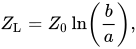
$Z_{\text{L}}$ = impedance of the feed transmission line (not shown).
$Z_{0}$ = impedance of free space.

The equation is the same as the equation for the impedance of a coaxial cable. However, a coaxial cable feed line is not assumed and not required.

The amplitude of the magnetic current density phasor is given by: ${\mathfrak {M}}^{\text{i}}={\frac {k}{\rho }}$ with $a\leq \rho \leq b.$ where

$\rho$ = radial distance from the axis.
$k={\frac {V_{\text{s}}}{\ln \left({\frac {b}{a}}\right)}}$ .
$V_{\text{s}}$ = magnitude of the source voltage phasor driving the feed line.

Watch videos about Magnetic currentExplainers and documentaries on YouTube (opens in a new tab)

Sources and credits

This article is adapted from the Wikipedia article “Magnetic current”, written by its contributors and licensed under CC BY-SA 4.0. Fathomly has changed the layout, removed citation markers, navigation and maintenance notices, and adjusted punctuation. This adapted version is shared under the same license. For references, see the original article.

Images, from Wikimedia Commons:

Magnetic Current Produces Electric Field By Left Hand Rule.svg by Constant314, CC BY-SA 4.0
Magnetic Frill Driving Dipole Antenna.png by Constant314, CC BY-SA 4.0

Fathomly is not affiliated with or endorsed by the Wikimedia Foundation. Spotted a problem? Tell us.