Reference articles on history, science, culture and more
Encyclopedia

Linear response function

Relationship of a signal transducer

A linear response function describes the input-output relationship of a signal transducer, such as a radio turning electromagnetic waves into music or a neuron turning synaptic input into a response. Because of its many applications in information theory, physics and engineering there exist alternative names for specific linear response functions such as susceptibility, impulse response or impedance; see also transfer function. The concept of a Green's function or fundamental solution of an ordinary differential equation is closely related.

01Mathematical definition

Denote the input of a system by h(t) (e.g. a force), and the response of the system by x(t) (e.g. a position). Generally, the value of x(t) will depend not only on the present value of h(t), but also on past values. Approximately x(t) is a weighted sum of the previous values of h(t'), with the weights given by the linear response function \chi (t-t'): x(t)=\int _{-\infty }^{t}dt'\,\chi (t-t')h(t')+\cdots \,.

The explicit term on the right-hand side is the leading order term of a Volterra expansion for the full nonlinear response. If the system in question is highly non-linear, higher order terms in the expansion, denoted by the dots, become important and the signal transducer cannot adequately be described just by its linear response function.

The complex-valued Fourier transform {\tilde {\chi }}(\omega ) of the linear response function is very useful as it describes the output of the system if the input is a sine wave h(t)=h_{0}\sin(\omega t) with frequency \omega. The output reads

x(t)=\left|{\tilde {\chi }}(\omega )\right|h_{0}\sin(\omega t+\arg {\tilde {\chi }}(\omega ))\,,

with amplitude gain |{\tilde {\chi }}(\omega )| and phase shift \arg {\tilde {\chi }}(\omega ).

02Example

Consider a damped harmonic oscillator with input given by an external driving force h(t),

{\ddot {x}}(t)+\gamma {\dot {x}}(t)+\omega _{0}^{2}x(t)=h(t).

The complex-valued Fourier transform of the linear response function is given by

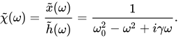
{\tilde {\chi }}(\omega )={\frac {{\tilde {x}}(\omega )}{{\tilde {h}}(\omega )}}={\frac {1}{\omega _{0}^{2}-\omega ^{2}+i\gamma \omega }}.

The amplitude gain is given by the magnitude of the complex number {\tilde {\chi }}(\omega ), and the phase shift by the arctan of the imaginary part of the function divided by the real one.

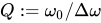
From this representation, we see that for small \gamma the Fourier transform {\tilde {\chi }}(\omega ) of the linear response function yields a pronounced maximum ("Resonance") at the frequency \omega \approx \omega _{0}. The linear response function for a harmonic oscillator is mathematically identical to that of an RLC circuit. The width of the maximum, \Delta \omega , typically is much smaller than \omega _{0}, so that the Quality factor Q:=\omega _{0}/\Delta \omega can be extremely large.

03Kubo formula

The exposition of linear response theory, in the context of quantum statistics, can be found in a paper by Ryogo Kubo. This defines particularly the Kubo formula, which considers the general case that the "force" h(t) is a perturbation of the basic operator of the system, the Hamiltonian, {\hat {H}}_{0}\to {\hat {H}}_{0}-h(t'){\hat {B}}(t') where {\hat {B}} corresponds to a measurable quantity as input, while the output x(t) is the perturbation of the thermal expectation of another measurable quantity {\hat {A}}(t). The Kubo formula then defines the quantum-statistical calculation of the susceptibility \chi (t-t') by a general formula involving only the mentioned operators.

As a consequence of the principle of causality the complex-valued function {\tilde {\chi }}(\omega ) has poles only in the lower half-plane. This leads to the Kramers-Kronig relations, which relates the real and the imaginary parts of {\tilde {\chi }}(\omega ) by integration. The simplest example is once more the damped harmonic oscillator.

04Nonequilibrium linear response formula

Linear response theory has versions for nonequilibrium processes for open systems where there is no detailed balance but a steady driving or agitation is applied. A small perturbation of these driven or active systems gives rise to a response in violation with the equilibrium expressions. A possible methodology proceeds via path-space ensembles where the probabilities of trajectories are evaluated; see e.g. The resulting response formulae have an entropic part (similar to the detailed balance case) and a frenetic part. The latter involves the correlation of the (excess) frenesy (due to the perturbation) with the observable. In detailed balance, the two contributions merge and reproduce the Kubo and Green-Kubo formulae. Out of detailed balance, the frenetic contribution is responsible for the possibility of negative heat capacities and mobilities, and they do not longer measure a fluctuation, e.g. in terms of a variance of the energy or of the current.

Watch videos about Linear response functionExplainers and documentaries on YouTube (opens in a new tab)

Sources and credits

This article is adapted from the Wikipedia article Linear response function, written by its contributors and licensed under CC BY-SA 4.0. Fathomly has changed the layout, removed citation markers, navigation and maintenance notices, and adjusted punctuation. This adapted version is shared under the same license. For references, see the original article.

Fathomly is not affiliated with or endorsed by the Wikimedia Foundation. Spotted a problem? Tell us.

Continue exploring

Related topics

Convolution

In mathematics, convolution is a mathematical operation on two functions f {\displaystyle f} and g {\displaystyle g} that produces a third function f ∗ g {\displaystyle f*g} , as the integral of the product of the two functions after one is reflected about the y-axis and shifted. The term convolution refers to both the resulting function and to the process of computing it.

Green-Kubo relations

The Green-Kubo relations give the exact mathematical expression for a transport coefficient γ {\displaystyle \gamma } in terms of the integral of the equilibrium time correlation function of the time derivative of a corresponding microscopic variable A {\displaystyle A} (sometimes termed a "gross variable", as in ): γ = ∫ 0 ∞ ⟨ A ˙ ( t ) A ˙ ( 0 ) ⟩ d t . {\displaystyle \gamma =\int _{0}^{\infty }\left\langle {\dot {A}}(t){\dot {A}}(0)\right\rangle \;{\mathrm {d} }t.} One intuitive way to understand this relation is that relaxations resulting from random fluctuations in equilibrium are indistinguishable from those due to an external perturbation in linear response.

Fluctuation theorem

The fluctuation theorem, which originated from statistical mechanics, deals with the relative probability that the entropy of a system which is currently away from thermodynamic equilibrium (i.e., maximum entropy) will increase or decrease over a given amount of time. While the second law of thermodynamics predicts that the entropy of an isolated system should tend to increase until it reaches equilibrium, it became apparent after the discovery of statistical mechanics that the second law is only a statistical one, suggesting that there should always be some nonzero probability that the entropy of an isolated system might spontaneously decrease; the fluctuation theorem precisely quantifies this probability.